1.3c: Adding topography to geological models

import gempy as gp
import numpy as np
import matplotlib.pyplot as plt
import os

1. The common procedure to set up a model:

data_path = 'https://raw.githubusercontent.com/cgre-aachen/gempy_data/master/'

geo_model = gp.create_model('Single_layer_topo')
gp.init_data(geo_model, extent=[450000, 460000, 70000, 80000, -1000, 500],
             resolution=[50, 50, 50],
             path_i=data_path + "/data/input_data/tut-ch1-7/onelayer_interfaces.csv",
             path_o=data_path + "/data/input_data/tut-ch1-7/onelayer_orient.csv")

Out:

Active grids: ['regular']

Single_layer_topo  2021-04-18 11:28

use happy spring colors!

geo_model.surfaces.colors.change_colors({'layer1': '#ff8000', 'basement': '#88cc60'})

gp.map_stack_to_surfaces(geo_model, {'series': ('layer1', 'basement')})

	surface	series	order_surfaces	color	id
0	layer1	series	1	#ff8000	1
1	basement	series	2	#88cc60	2

s = {'s1': ([450000, 75000], [460000, 75500], [100, 100])}
geo_model.set_section_grid(s)

Out:

Active grids: ['regular' 'sections']

	start	stop	resolution	dist
s1	[450000, 75000]	[460000, 75500]	[100, 100]	10012.49

2. Adding topography

2 a. Load from raster file

This is to make it work in sphinx gallery

cwd = os.getcwd()
if not 'examples' in cwd:
    path_dir = os.getcwd() + '/examples/tutorials/ch5_probabilistic_modeling'
else:
    path_dir = cwd

fp = path_dir + "/../../data/input_data/tut-ch1-7/bogota.tif"

geo_model.set_topography(source='gdal', filepath=fp)
gp.plot_2d(geo_model, show_topography=True, section_names=['topography'], show_lith=False,
           show_boundaries=False,
           kwargs_topography={'cmap': 'gray', 'norm': None}
           )
plt.show()

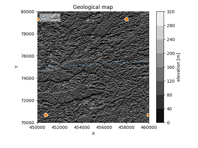
Out:

Cropped raster to geo_model.grid.extent.
depending on the size of the raster, this can take a while...
storing converted file...
Active grids: ['regular' 'topography' 'sections']

2 b. create fun topography

If there is no topography file, but you think that your model with topography would look significantly cooler, you can use gempys set_topography function to generate a random topography based on a fractal grid:

sphinx_gallery_thumbnail_number = 2

geo_model.set_topography(source='random')
gp.plot_2d(geo_model, show_topography=True, section_names=['topography'])
plt.show()

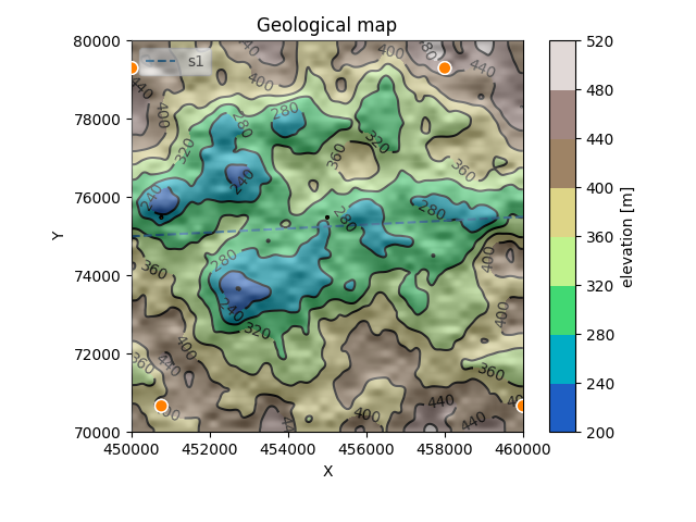
Out:

[200. 500.]
Active grids: ['regular' 'topography' 'sections']

It has additional keywords to play around with:

• fd: fractal dimension:

  defaults to 2.0. The higher (try 2.9), the rougher the landscape will be.

• d_z: height difference:

  If none, last 20% of the model in z direction.

• extent:

  extent in xy direction. If none, geo_model.grid.extent is used.

• resolution:

  resolution of the topography array. If none, geo_model.grid.resoution is used. Increasing the resolution leads to much nicer geological maps!

geo_model.set_topography(source='random', fd=1.9, d_z=np.array([0, 250]),
                         resolution=np.array([200, 200]))

Out:

Active grids: ['regular' 'topography' 'sections']

Grid Object. Values:
array([[450100.        ,  70100.        ,   -985.        ],
       [450100.        ,  70100.        ,   -955.        ],
       [450100.        ,  70100.        ,   -925.        ],
       ...,
       [460000.        ,  75500.        ,    469.6969697 ],
       [460000.        ,  75500.        ,    484.84848485],
       [460000.        ,  75500.        ,    500.        ]])

Note that each time this function is called, a new random topography is created. If you particularly like the generated topography or if you have loaded a large file with gdal, you can save the topography object and load it again later:

save:

geo_model._grid.topography.save('test_topo')

load:

geo_model.set_topography(source='saved', filepath='test_topo.npy')

Out:

Active grids: ['regular' 'topography' 'sections']

Grid Object. Values:
array([[450100.        ,  70100.        ,   -985.        ],
       [450100.        ,  70100.        ,   -955.        ],
       [450100.        ,  70100.        ,   -925.        ],
       ...,
       [460000.        ,  75500.        ,    469.6969697 ],
       [460000.        ,  75500.        ,    484.84848485],
       [460000.        ,  75500.        ,    500.        ]])

Compute model

gp.set_interpolator(geo_model)

Out:

Setting kriging parameters to their default values.
Compiling theano function...
Level of Optimization:  fast_compile
Device:  cpu
Precision:  float64
Number of faults:  0
Compilation Done!
Kriging values:
                      values
range              14221.46
$C_o$            4815476.19
drift equations         [3]

<gempy.core.interpolator.InterpolatorModel object at 0x7fcb8ae537f0>

gp.compute_model(geo_model, compute_mesh=False, set_solutions=True)

Out:

Lithology ids
  [2. 2. 2. ... 1. 1. 1.]

Visualize:

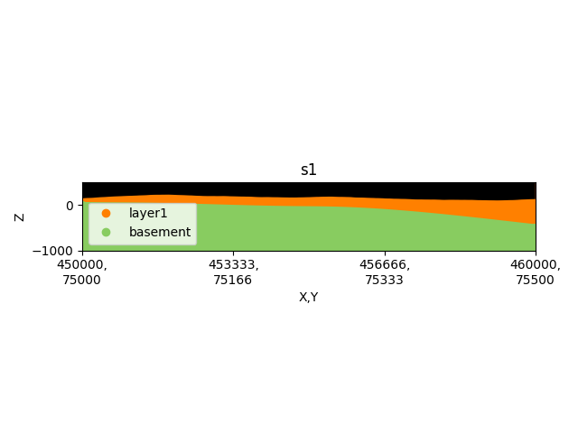
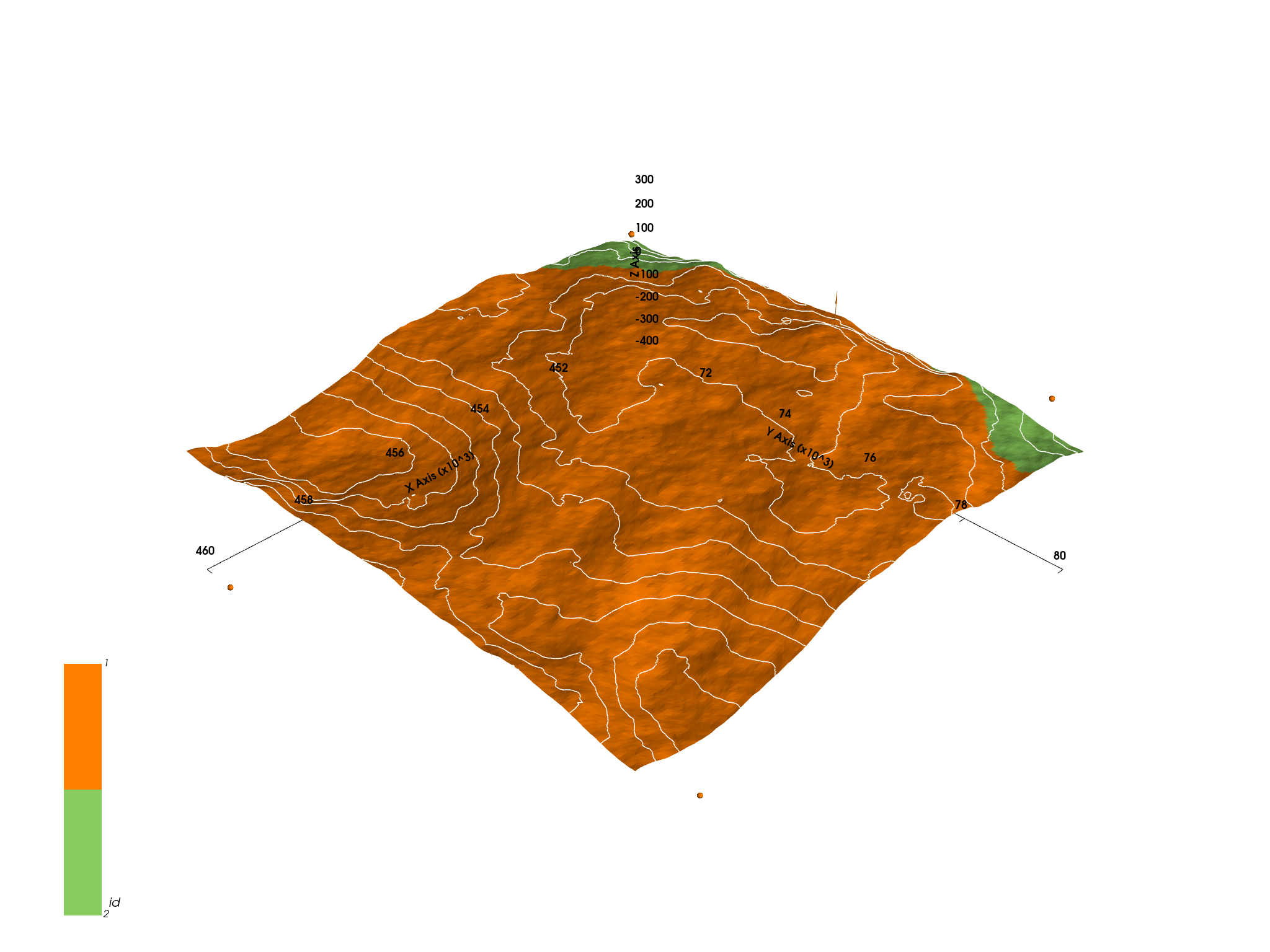
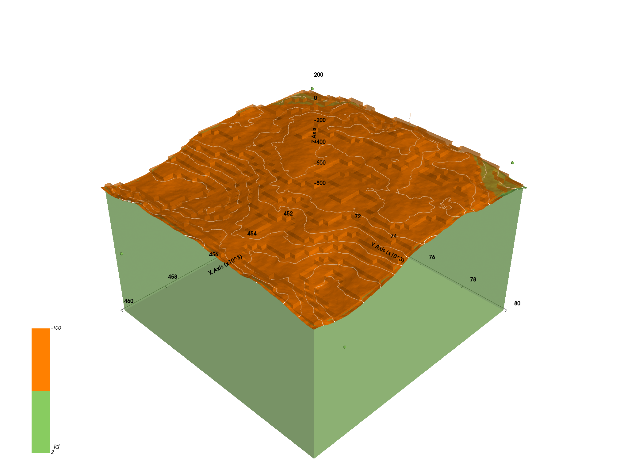
Now, the solutions object does also contain the computed geological map. It can be visualized using the 2D and 3D plotting functionality:

gp.plot_2d(geo_model, show_topography=True, section_names=['topography'], show_boundaries=False, show_data=True)
plt.show()

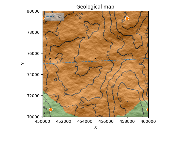
gp.plot_2d(geo_model, show_topography=True, section_names=['s1'])
plt.show()

g3d = gp.plot_3d(geo_model,
                 show_topography=True,
                 show_lith=False,
                 show_surfaces=False,
                 show_results=False,
                 ve=5)

sphinx_gallery_thumbnail_number = 3

g3d = gp.plot_3d(geo_model,
                 show_topography=True,
                 show_lith=True,
                 show_surfaces=True,
                 ve=5)