Model 1 - Reading GeoTop Data

This tutorial demonstrates how to read borehole data using GeoTop and set up the stratigraphic pile using GemPy.

Step 1: Import Necessary Libraries

Here we import the libraries necessary for handling the environment variables, numerical operations, data handling with pandas, and the specific functions from subsurface and gempy packages.

import dotenv
import os
import numpy as np
import pandas as pd
import subsurface
import gempy as gp
from gempy_geotop.model_constructor import initialize_geomodel, add_fault_from_unstructured_data
from gempy_geotop.geotop_stratigraphy import stratigraphy_pile, color_elements
from gempy_geotop.reader import read_all_boreholes_data_to_df, read_all_fault_data_to_mesh, add_raw_faults_to_mesh
from gempy_geotop.utils import plot_geotop

Step 2: Load Environment Variables

Environment variables are a secure way to manage configurations and sensitive data. Here we load the environment variables that specify the path to the borehole data.

dotenv.load_dotenv()

True

Step 3: Read Borehole Data

We read the borehole data from the specified directory. This data will be used to initialize and configure the geological model in GemPy.

data_south: pd.DataFrame = read_all_boreholes_data_to_df(
    path=os.getenv('BOREHOLES_SOUTH_FOLDER')
)

Step 4: Initialize GemPy Model

Using the borehole data, we initialize the GemPy model. We also slice the formations to consider only the first 10, adjusting the model’s complexity and processing time.

geo_model = initialize_geomodel(data_south)
slice_formations = slice(0, 10)  # Slice the formations to the first 10
depth = -500.0  # Define a fixed depth for the model's base

[120071, 209998, 370060, 419970, -901.5, 48.68]

Step 5: Map Stratigraphy and Color Elements

Here we map the stratigraphy pile to the GemPy model and assign colors to different geological units for better visualization.

gp.map_stack_to_surfaces(
    gempy_model=geo_model,
    mapping_object=stratigraphy_pile
)
color_elements(geo_model.structural_frame.structural_elements)

Could not find element 'VE' in any group.
Could not find element 'RU' in any group.
Could not find element 'TO' in any group.
Could not find element 'DO' in any group.
Could not find element 'LA' in any group.
Could not find element 'HT' in any group.
Could not find element 'HO' in any group.
Could not find element 'MT' in any group.
Could not find element 'GU' in any group.
Could not find element 'VA' in any group.
Could not find element 'AK' in any group.

Step 6: Configure and Set Grid

We set up the grid for the model, defining its spatial extent and resolution based on the surface points and a specified depth.

geo_model.structural_frame.structural_groups = geo_model.structural_frame.structural_groups[slice_formations]
xyz = geo_model.surface_points_copy.xyz

extent = [
        xyz[:, 0].min(), xyz[:, 0].max(),
        xyz[:, 1].min(), xyz[:, 1].max(),
        depth, xyz[:, 2].max()
]

geo_model.grid.regular_grid.set_regular_grid(
    extent=extent,
    resolution=np.array([50, 50, 50])
)

array([[ 1.2097027e+05,  3.7055910e+05, -4.9451320e+02],
       [ 1.2097027e+05,  3.7055910e+05, -4.8353960e+02],
       [ 1.2097027e+05,  3.7055910e+05, -4.7256600e+02],
       ...,
       [ 2.0909873e+05,  4.1947090e+05,  2.1246000e+01],
       [ 2.0909873e+05,  4.1947090e+05,  3.2219600e+01],
       [ 2.0909873e+05,  4.1947090e+05,  4.3193200e+01]])

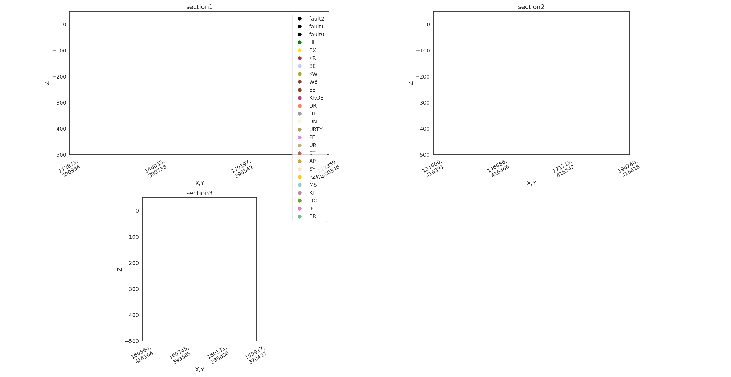
Step 7: Set Sections for Visualization

We define specific sections of the model for detailed visualization. These sections help in analyzing the model from different perspectives and depths.

gp.set_section_grid(
    grid=geo_model.grid,
    section_dict={
            'section1': ([112873, 390934], [212359, 390346], [100, 100]),
            'section2': ([121660, 416391], [196740, 416618], [100, 100]),
            'section3': ([160560, 414164], [159917, 370427], [100, 100])
    }
)

Active grids: ['sections']

	start	stop	resolution	dist
section1	[112873, 390934]	[212359, 390346]	[100, 100]	99487.737636
section2	[121660, 416391]	[196740, 416618]	[100, 100]	75080.343160
section3	[160560, 414164]	[159917, 370427]	[100, 100]	43741.726281

Step 8: Read and Process Fault Data

We read fault data, slice it for processing the first few entries, and integrate these faults into the geological model.

all_unstruct: list[subsurface.UnstructuredData] = read_all_fault_data_to_mesh(
    path=os.getenv('FAULTS_SOUTH_FOLDER')
)

slice_faults = slice(0, 3)  # Slice the faults to the first 3 for simplicity
subset = all_unstruct[slice_faults]  # Take the first 3 faults

for e, struct in enumerate(subset):
    add_fault_from_unstructured_data(
        unstruct=struct,
        geo_model=geo_model,
        name=f"fault{e}"
    )

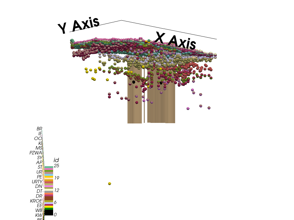
Step 9: Visualize the Model

Finally, we plot the 3D visualization of the geological model, showing both the stratigraphy and the faults. Adjust the vertical exaggeration for better depth perception.

plot_3d = plot_geotop(geo_model, ve=100, image_3d=False, show=False)
add_raw_faults_to_mesh(subset, plot_3d)
plot_3d.p.show()