Model 2 - Computing Model

This tutorial covers the steps required to compute a geological model using GemPy, including setup, computation, and visualization.

Step 1: Import Necessary Libraries

Importing the required libraries for environmental variable management, model generation, and visualization.

import dotenv
from gempy_geotop.example_models import generate_south_model_base
import gempy as gp
import gempy_viewer as gpv

Step 2: Load Environment Variables

Loading environment variables which may include paths or configurations necessary for the model generation.

dotenv.load_dotenv()

True

Step 3: Generate Base Geological Model

We start by generating a base geological model using predefined settings. This function might configure basic layers, fault systems, and other geological parameters based on the southern region model.

geo_model = generate_south_model_base(group_slicer=slice(0, 10))

[120071, 209998, 370060, 419970, -901.5, 48.68]
Could not find element 'KR' in any group.
Could not find element 'KW' in any group.
Could not find element 'WB' in any group.
Could not find element 'EE' in any group.
Could not find element 'KROE' in any group.
Could not find element 'DR' in any group.
Could not find element 'DT' in any group.
Could not find element 'DN' in any group.
Could not find element 'URTY' in any group.
Could not find element 'PE' in any group.
Could not find element 'UR' in any group.
Could not find element 'AP' in any group.
Could not find element 'IE' in any group.
Could not find element 'VE' in any group.
Could not find element 'RU' in any group.
Could not find element 'TO' in any group.
Could not find element 'DO' in any group.
Could not find element 'LA' in any group.
Could not find element 'HT' in any group.
Could not find element 'HO' in any group.
Could not find element 'MT' in any group.
Could not find element 'GU' in any group.
Could not find element 'VA' in any group.
Could not find element 'AK' in any group.
Active grids: ['sections']

Step 4: Configure Interpolation Options

Setting the cache mode to CACHE to optimize interpolation calculations during model computation. This improves performance especially for complex models.

geo_model.interpolation_options.cache_mode = gp.data.InterpolationOptions.CacheMode.CACHE

Step 5: Compute the Geological Model

Computing the geological model using NumPy backend. We also enable GPU acceleration to further enhance the computation speed. The data type used is float64 for high precision.

gp.compute_model(
    gempy_model=geo_model,
    engine_config=gp.data.GemPyEngineConfig(
        backend=gp.data.AvailableBackends.numpy,
        use_gpu=True,
        dtype='float64'
    )
)

Setting Backend To: AvailableBackends.numpy
A size: (1907, 1907)
CG iterations: 461
A size: (1692, 1692)
CG iterations: 420
A size: (1365, 1365)
CG iterations: 338
A size: (1269, 1269)
CG iterations: 397
A size: (1087, 1087)
CG iterations: 286
A size: (1040, 1040)
CG iterations: 343
A size: (614, 614)
CG iterations: 282
A size: (489, 489)
CG iterations: 232
A size: (22, 22)
CG iterations: 45

Solutions: 4 Octree Levels, 10 DualContouringMeshes

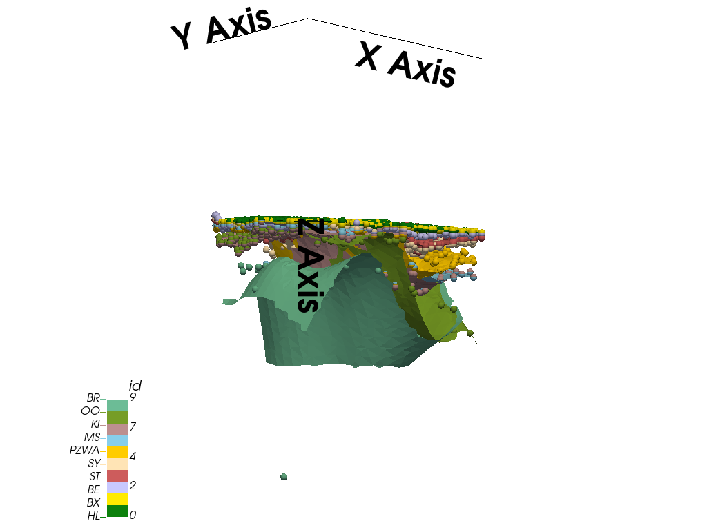
Step 6: Visualize the Model in 3D

Creating a 3D visualization of the geological model using GemPy Viewer. We customize the view to show certain data elements and adjust aesthetics like opacity and labels visibility.

ve = 100  # Vertical exaggeration for better depth perception
gempy_plot3d = gpv.plot_3d(
    model=geo_model,
    show_data=True,
    show_lith=False,
    ve=ve,
    image=False,
    kwargs_pyvista_bounds={
            'show_xlabels': False,
            'show_ylabels': False,
            'show_zlabels': False,
    },
    kwargs_plot_data={'arrow_size': 100},
    kwargs_plot_structured_grid={'opacity': .8}
)

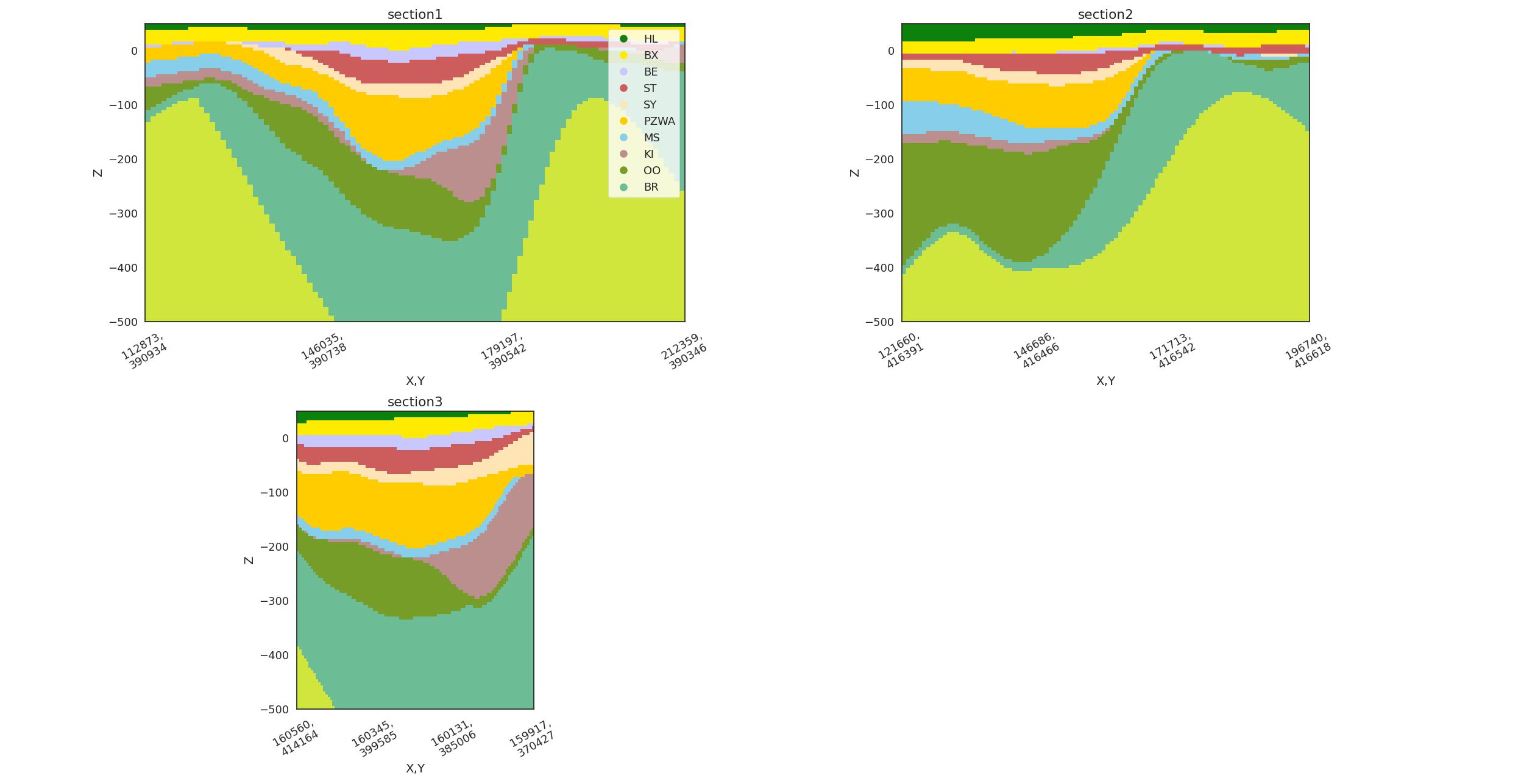
Step 7: Create 2D Cross-Sections

In addition to 3D visualization, we generate 2D cross-sections of the model. This includes multiple sections to provide detailed views at different angles. Vertical exaggeration and projection distances are configured to enhance the visual output.

# sphinx_gallery_thumbnail_number = 2
gpv.plot_2d(
    model=geo_model,
    section_names=['section1', 'section2', 'section3'],
    show_data=True,
    show_boundaries=False,
    ve=ve,
    projection_distance=100
)

<gempy_viewer.modules.plot_2d.visualization_2d.Plot2D object at 0x7facc6093b80>