Hecho

These two lines are necessary only if gempy is not installed

import sys, os
import urllib

os.environ["THEANO_FLAGS"] = "mode=FAST_RUN,device=cpu"
# Importing gempy
import gempy as gp

# Aux imports
import numpy as np
import pandas as pn
import matplotlib.pyplot as plt

Loading surface points from repository:

With pandas we can do it directly from the web and with the right args we can directly tidy the data in gempy style:

dfs = []
data_amount = 'Full'

# First stratigraphic data
for letter in range(1, 10):

    try:
        dfs.append(pn.read_csv('https://raw.githubusercontent.com/Loop3D/ImplicitBenchmark/master'
                               f'/Hecho/{data_amount}/H' +
                               str(letter) + '.csv', sep=';',
                               names=['X', 'Y', 'Z', 'surface', '_'], header=0))
    except urllib.error.HTTPError as e:
        print(e, letter)

# Also faults
for f in range(1, 4):
    fault_df = pn.read_csv('https://raw.githubusercontent.com/Loop3D/ImplicitBenchmark/master/Hecho/F' +
                           str(f) + 'Line.csv',
                           sep=';', names=['X', 'Y', 'Z'], header=0)
    fault_df['surface'] = 'f' + str(f)
    dfs.append(fault_df)

# We put all the surfaces points together because is how gempy likes it:
surface_points = pn.concat(dfs, sort=True)
surface_points.reset_index(inplace=True, drop=False)
surface_points.tail()

	index	X	Y	Z	_	surface
761	6	11.14	-0.17	1.53	NaN	f3
762	7	11.17	0.28	1.68	NaN	f3
763	8	11.16	0.40	1.82	NaN	f3
764	9	11.07	0.03	1.92	NaN	f3
765	10	10.89	-0.43	2.10	NaN	f3

Now we do the same with the orientations:

orientations = pn.read_csv('https://raw.githubusercontent.com/Loop3D/ImplicitBenchmark/master/Hecho/Sparse/Dips.csv',
                           sep=';',
                           names=['X', 'Y', 'Z', 'G_x', 'G_z', '_'], header=0)
# Orientation needs to belong to a surface. This is mainly to categorize to which series belong and to
# use the same color
orientations['surface'] = 0

# We fill the laking direction with a dummy value:
orientations['G_y'] = 0

# Drop unecesary data point
orientations.drop([1, 3, 4], inplace=True)
orientations

	X	Y	Z	G_x	G_z	_	surface	G_y
0	3.81	0.16	0.58	0.62	0.79	4	0	0
2	9.87	0.06	2.52	-0.76	0.64	20	0	0
5	4.83	-0.03	3.33	0.07	1.00	28	0	0

Data initialization:

Suggested size of the axis-aligned modeling box: Origin: 0 -0.5 0 Maximum: 16 0.5 4.5

Suggested resolution: 0.05m (grid size 321 x 21 x 91)

geo_model = gp.create_model('Moureze')
geo_model = gp.init_data(geo_model, extent=[0, 16, -0.5, 0.5, 0, 4.5], resolution=[321, 21, 91],
                         surface_points_df=surface_points, orientations_df=orientations,
                         surface_name='surface',
                         add_basement=True)

Out:

Active grids: ['regular']

geo_model.orientations.df.at[5, 'surface']

Out:

0

geo_model.orientations.df

	X	Y	Z	X_c	Y_c	Z_c	G_x	G_y	G_z	dip	azimuth	polarity	surface	series	id	order_series	smooth
0	3.81	0.16	0.58	0.37	0.51	0.45	0.62	0.0	0.79	38.25	90.0	1	0	Default series	1	1	0.01
2	9.87	0.06	2.52	0.57	0.50	0.51	-0.76	0.0	0.64	49.86	270.0	1	0	Default series	1	1	0.01
5	4.83	-0.03	3.33	0.40	0.50	0.54	0.07	0.0	1.00	3.89	90.0	1	0	Default series	1	1	0.01

We need an orientation per series/fault. The faults does not have orientation so the easiest is to create an orientation from the surface points availablle:

f_names = ['f1', 'f2', 'f3']
for fn in f_names:
    fault_idx = geo_model.surface_points.df.index[geo_model.surface_points.df['surface'] == fn]
    gp.set_orientation_from_surface_points(geo_model, fault_idx)

Now we can see how the data looks so far:

gp.plot_2d(geo_model)

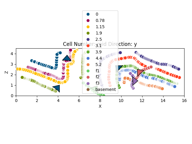
Out:

<gempy.plot.visualization_2d.Plot2D object at 0x7fccd1ea9970>

By default all surfaces belong to one unique series.

geo_model.surfaces

	surface	series	order_surfaces	color	id
0	0	Default series	1	#015482	1
1	0.78	Default series	2	#9f0052	2
2	1.15	Default series	3	#ffbe00	3
3	1.90	Default series	4	#728f02	4
4	2.50	Default series	5	#443988	5
5	3.10	Default series	6	#ff3f20	6
6	3.90	Default series	7	#5DA629	7
7	4.40	Default series	8	#4878d0	8
8	5.20	Default series	9	#ee854a	9
9	f1	Default series	10	#6acc64	10
10	f2	Default series	11	#d65f5f	11
11	f3	Default series	12	#956cb4	12
12	basement	Basement	1	#8c613c	13

geo_model.orientations.df.dtypes

Out:

X                float64
Y                float64
Z                float64
X_c              float64
Y_c              float64
Z_c              float64
G_x              float64
G_y              float64
G_z              float64
dip              float64
azimuth          float64
polarity           int64
surface         category
series          category
id                 int64
order_series       int64
smooth           float64
dtype: object

We will need to separate with surface belong to each series:

gp.map_stack_to_surfaces(geo_model, {'Fault1': 'f1', 'Fault2': 'f2', 'Fault3': 'f3'})

	surface	series	order_surfaces	color	id
0	0	Default series	1	#015482	1
1	0.78	Default series	2	#9f0052	2
2	1.15	Default series	3	#ffbe00	3
3	1.90	Default series	4	#728f02	4
4	2.50	Default series	5	#443988	5
5	3.10	Default series	6	#ff3f20	6
6	3.90	Default series	7	#5DA629	7
7	4.40	Default series	8	#4878d0	8
8	5.20	Default series	9	#ee854a	9
9	f1	Fault1	1	#6acc64	10
10	f2	Fault2	1	#d65f5f	11
11	f3	Fault3	1	#956cb4	12
12	basement	Basement	1	#8c613c	13

However if we want the faults to offset the “Default series”, they will need to be more recent (higher on the pile). We can modify the order by:

geo_model.modify_order_series(4, 'Default series')

	order_series	BottomRelation	isActive	isFault	isFinite
Fault3	1	Erosion	True	False	False
Fault1	2	Erosion	True	False	False
Fault2	3	Erosion	True	False	False
Default series	4	Erosion	True	False	False
Basement	5	Erosion	False	False	False

Lastly, so far we did not specify which series/faults are actula faults:

geo_model.set_is_fault(['Fault1', 'Fault2', 'Fault3'])

Out:

Fault colors changed. If you do not like this behavior, set change_color to False.

	order_series	BottomRelation	isActive	isFault	isFinite
Fault3	1	Fault	True	True	False
Fault1	2	Fault	True	True	False
Fault2	3	Fault	True	True	False
Default series	4	Erosion	True	False	False
Basement	5	Erosion	False	False	False

Now we are good to go:

gp.set_interpolator(geo_model, theano_optimizer='fast_run', dtype='float64')

Out:

Setting kriging parameters to their default values.
Compiling theano function...
Level of Optimization:  fast_run
Device:  cpu
Precision:  float64
Number of faults:  3
Compilation Done!
Kriging values:
                           values
range                      16.65
$C_o$                        6.6
drift equations  [3, 3, 3, 3, 3]

<gempy.core.interpolator.InterpolatorModel object at 0x7fcb8b176eb0>

The default range is always the diagonal of the extent. Since in this model data is very close we will need to reduce the range to 5-10% of that value:

new_range = geo_model.get_additional_data().loc[('Kriging', 'range'), 'values'] * 0.2
geo_model.modify_kriging_parameters('range', new_range)

	values
range	3.33
$C_o$	6.6
drift equations	[3, 3, 3, 3, 3]

gp.compute_model(geo_model, sort_surfaces=True, compute_mesh=False)

Out:

Lithology ids
  [10.         10.         10.         ... 10.          9.99645237
  8.09615495]

Time

• GTX 2080 164 ms ± 2.03 ms per loop (mean ± std. dev. of 7 runs, 1 loop each)

gp.plot_2d(geo_model, cell_number=[10], series_n=3, show_scalar=True)

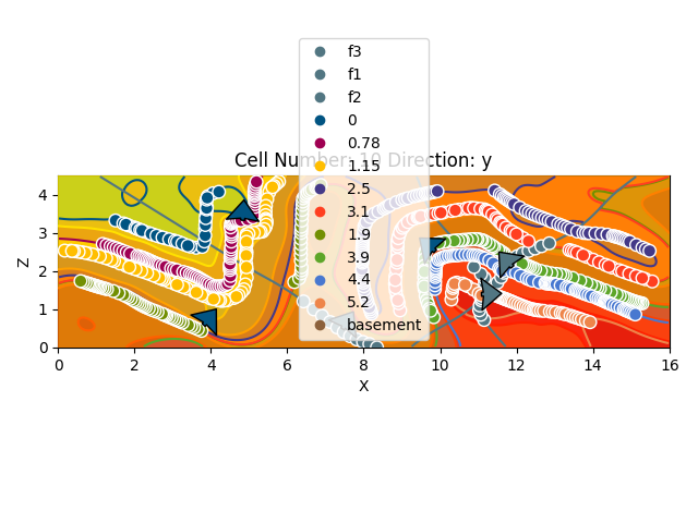
Out:

<gempy.plot.visualization_2d.Plot2D object at 0x7fcc3c7aaee0>

gp.plot_2d(geo_model, cell_number=[10], show_data=True)

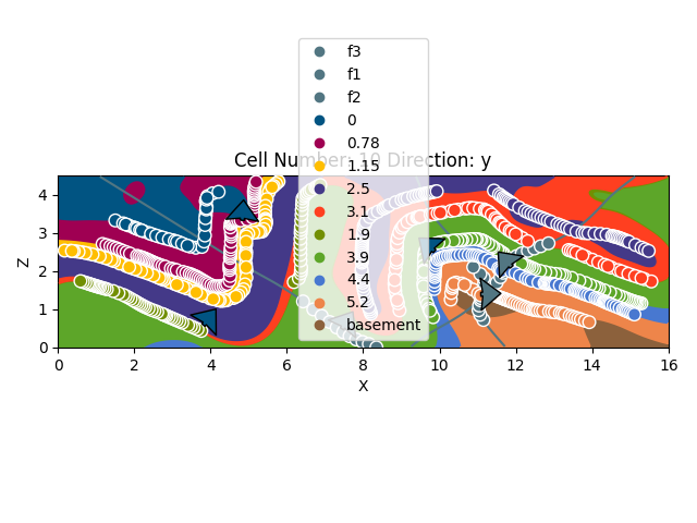
Out:

<gempy.plot.visualization_2d.Plot2D object at 0x7fcb8b8b5970>

sphinx_gallery_thumbnail_number = 3

gp.plot_3d(geo_model, kwargs_plot_structured_grid={'opacity': 8})

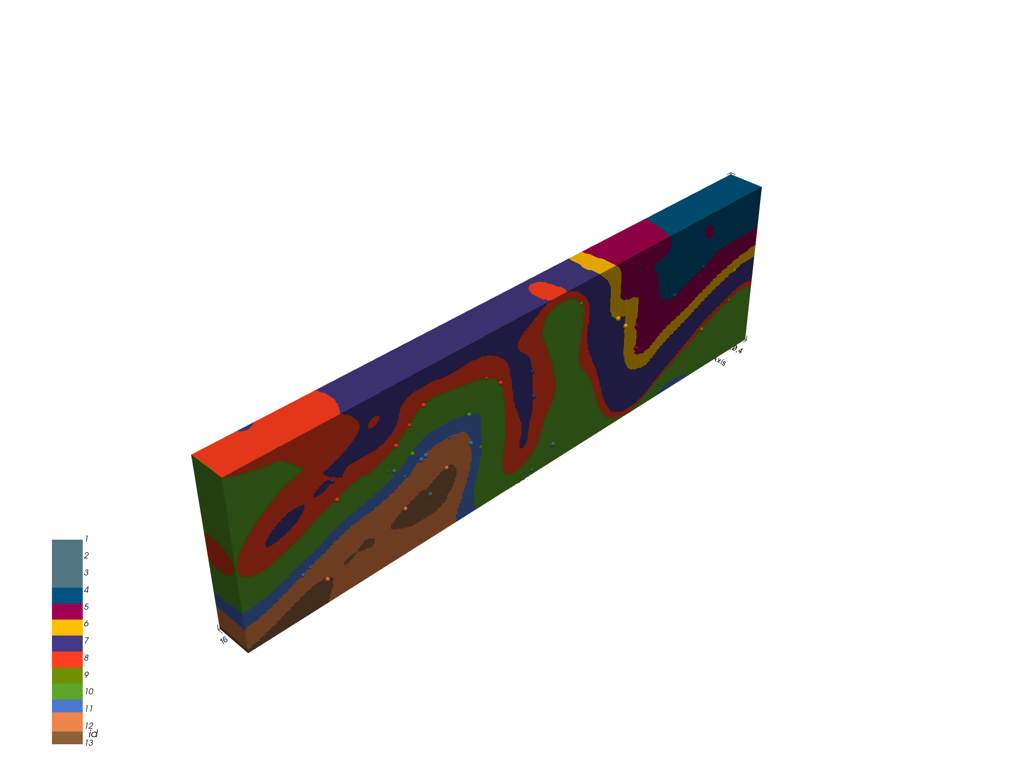
Out:

<gempy.plot.vista.GemPyToVista object at 0x7fcc46b3f1f0>

Export data:

The solution is stored in a numpy array of the following shape. Axis 0 are the scalar fields of each correspondent series/faults in the following order (except basement):

geo_model.series

	order_series	BottomRelation	isActive	isFault	isFinite
Fault3	1	Fault	True	True	False
Fault1	2	Fault	True	True	False
Fault2	3	Fault	True	True	False
Default series	4	Erosion	True	False	False
Basement	5	Erosion	False	False	False

For the surfaces, there are two numpy arrays, one with vertices and the other with triangles. Axis 0 is each surface in the order:

geo_model.surfaces

	surface	series	order_surfaces	color	id
11	f3	Fault3	1	#527682	1
9	f1	Fault1	1	#527682	2
10	f2	Fault2	1	#527682	3
0	0	Default series	1	#015482	4
1	0.78	Default series	2	#9f0052	5
2	1.15	Default series	3	#ffbe00	6
4	2.50	Default series	4	#443988	7
5	3.10	Default series	5	#ff3f20	8
3	1.90	Default series	6	#728f02	9
6	3.90	Default series	7	#5DA629	10
7	4.40	Default series	8	#4878d0	11
8	5.20	Default series	9	#ee854a	12
12	basement	Basement	1	#8c613c	13

np.save('Hecho_scalar', geo_model.solutions.scalar_field_matrix)

def write_property_to_gocad_voxet(propertyfilename, propertyvalues):
    """
    This function writes a numpy array into the right format for a gocad
    voxet property file. This assumet there is a property already added to the .vo file,
    and is just updating the file.
    propertyfile - string giving the path to the file to write
    propertyvalues - numpy array nz,ny,nx ordering and in float format
    """
    propertyvalues = propertyvalues.astype('>f4')  # big endian
    #     array = propertyvalues.newbyteorder()
    propertyvalues.tofile(propertyfilename)

write_property_to_gocad_voxet(f'hecho_sf_gempy_{data_amount}',
                              geo_model.solutions.scalar_field_matrix[3].reshape([321, 21, 91]).ravel('F'))

4

Out:

4