2.2: Centered Grid.

Geophysics Preprocessing builds on the centered grid (https://github.com/cgre-aachen/gempy/blob/master/notebooks/tutorials/ch1-3-Grids.ipynb) to precompute the constant part of forward physical computations as for example gravity:

\[F_z = G_{\rho} ||| x \ln(y+r) + y \ln (x+r) - z \arctan (\frac{x y}{z r}) |^{x_2}_{x_1}|^{y_2}_{y_1}|^{ z_2}_{z_1}\]

where we can compress the grid dependent terms as

\[t_z = ||| x \ln (y+r) + y \ln (x+r)-z \arctan ( \frac{x y}{z r} ) |^{x_2}_{x_1}|^{y_2}_{y_1}|^{z_2}_{z_1}\]

By doing this decomposition an keeping the grid constant we can compute the forward gravity by simply operate:

\[F_z = G_{\rho} \cdot t_z\]

# Importing gempy
from gempy.assets.geophysics import GravityPreprocessing

# Aux imports
import numpy as np
import pandas as pd
import matplotlib.pyplot as plt

np.random.seed(1515)
pd.set_option('precision', 2)

g = GravityPreprocessing()

kernel_centers, kernel_dxyz_left, kernel_dxyz_right = g.create_irregular_grid_kernel(resolution=[10, 10, 20],
                                                                                     radius=100)

create_irregular_grid_kernel will create a constant kernel around the point 0,0,0. This kernel will be what we use for each device.

kernel_centers

Out:

array([[-100.        , -100.        ,   -6.        ],
       [-100.        , -100.        ,   -7.2       ],
       [-100.        , -100.        ,   -7.52912998],
       ...,
       [ 100.        ,  100.        ,  -79.90178533],
       [ 100.        ,  100.        , -100.17119644],
       [ 100.        ,  100.        , -126.        ]])

\(t_z\) is only dependent on distance and therefore we can use the kerenel created on the previous cell

tz = g.set_tz_kernel(resolution=[10, 10, 20], radius=100)
tz

Out:

array([-8.71768928e-05, -6.45647022e-05, -3.41579985e-05, ...,
       -1.09610058e-02, -1.41543038e-02, -1.51096613e-02])

To compute tz we also need the edges of each voxel. The distance to the edges are stored on kernel_dxyz_left and kernel_dxyz_right. We can plot all the data as follows:

a, b, c = kernel_centers, kernel_dxyz_left, kernel_dxyz_right

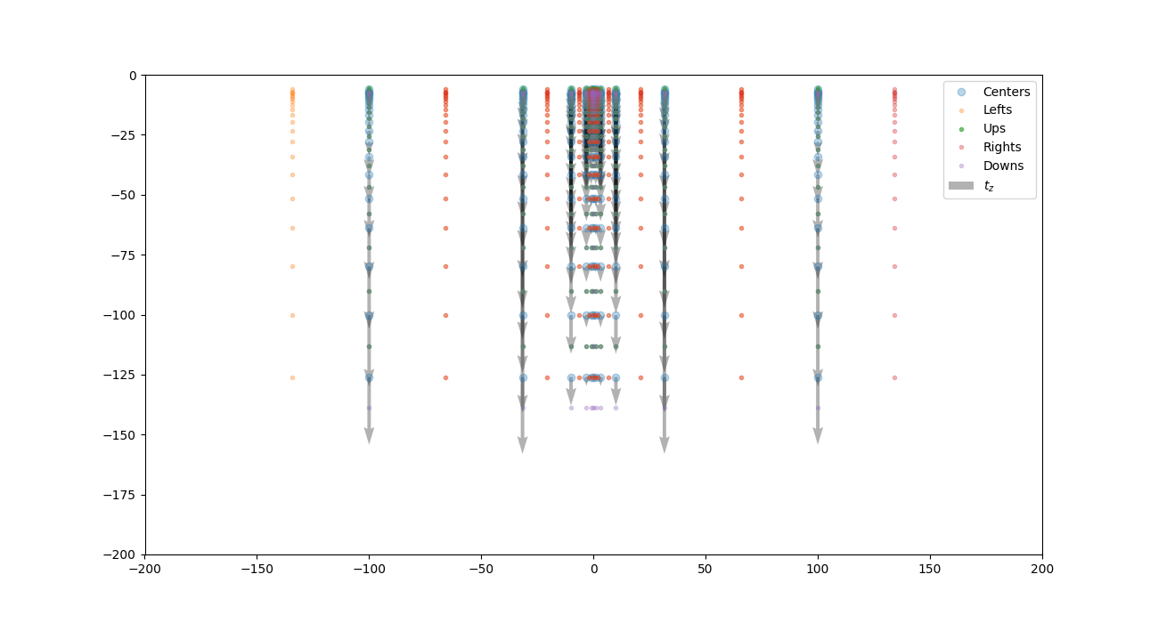
fig = plt.figure(figsize=(13, 7))
plt.quiver(a[:, 0].reshape(11, 11, 21)[5, :, :].ravel(),
           a[:, 2].reshape(11, 11, 21)[:, 5, :].ravel(),
           np.zeros(231),
           tz.reshape(11, 11, 21)[5, :, :].ravel(), label='$t_z$', alpha=.3
           )

plt.plot(a[:, 0].reshape(11, 11, 21)[5, :, :].ravel(),
         a[:, 2].reshape(11, 11, 21)[:, 5, :].ravel(), 'o', alpha=.3, label='Centers')

plt.plot(a[:, 0].reshape(11, 11, 21)[5, :, :].ravel() - b[:, 0].reshape(11, 11, 21)[5, :, :].ravel(),
         a[:, 2].reshape(11, 11, 21)[:, 5, :].ravel(), '.', alpha=.3, label='Lefts')

plt.plot(a[:, 0].reshape(11, 11, 21)[5, :, :].ravel(),
         a[:, 2].reshape(11, 11, 21)[:, 5, :].ravel() - b[:, 2].reshape(11, 11, 21)[:, 5, :].ravel(), '.', alpha=.6,
         label='Ups')

plt.plot(a[:, 0].reshape(11, 11, 21)[5, :, :].ravel() + c[:, 0].reshape(11, 11, 21)[5, :, :].ravel(),
         a[:, 2].reshape(11, 11, 21)[:, 5, :].ravel(), '.', alpha=.3, label='Rights')

plt.plot(a[:, 0].reshape(11, 11, 21)[5, :, :].ravel(),
         a[:, 2].reshape(11, 11, 21)[:, 5, :].ravel() + c[:, 2].reshape(11, 11, 21)[5, :, :].ravel(), '.', alpha=.3,
         label='Downs')

plt.xlim(-200, 200)
plt.ylim(-200, 0)
plt.legend()
plt.show()

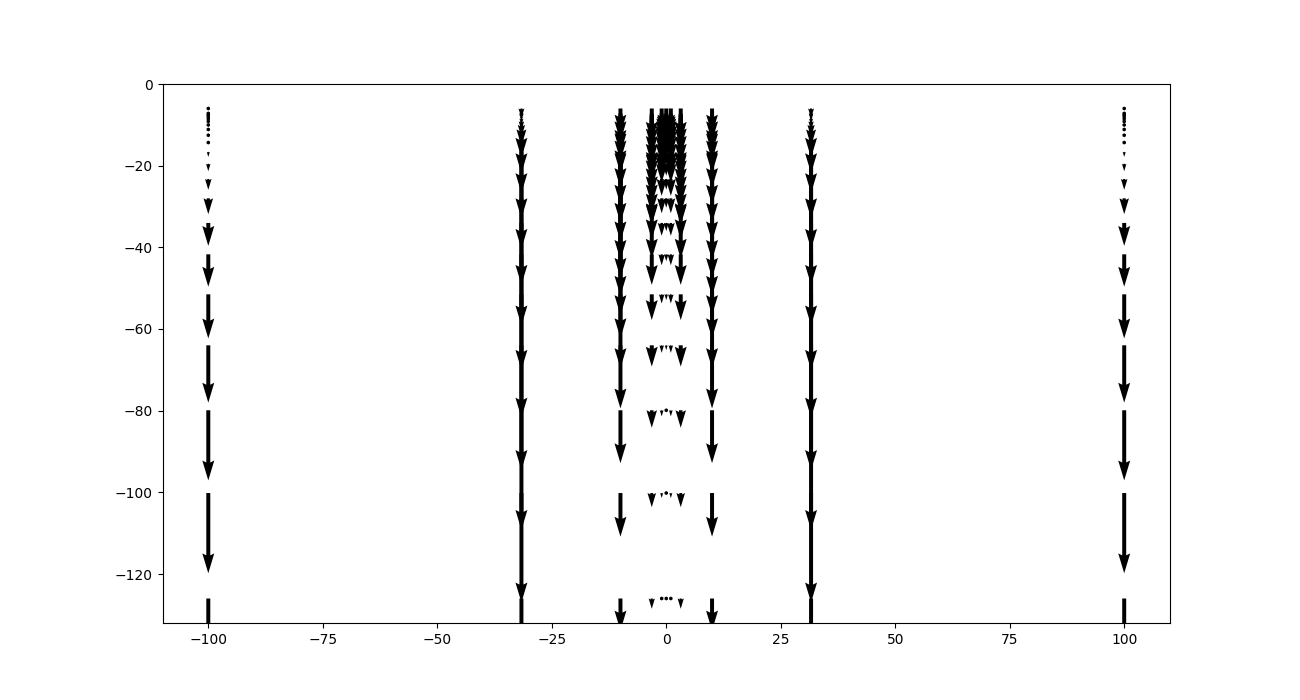
Just the quiver:

fig = plt.figure(figsize=(13, 7))
plt.quiver(a[:, 0].reshape(11, 11, 21)[5, :, :].ravel(),
           a[:, 2].reshape(11, 11, 21)[:, 5, :].ravel(),
           np.zeros(231),
           tz.reshape(11, 11, 21)[5, :, :].ravel()
           )
plt.show()

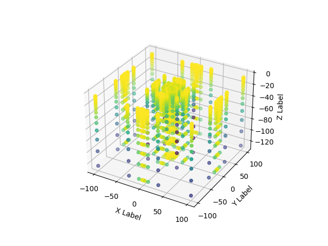
Remember this is happening always in 3D:

fig = plt.figure()
ax = fig.add_subplot(111, projection='3d')

ax.scatter(a[:, 0], a[:, 1], a[:, 2], c=tz)

ax.set_xlabel('X Label')
ax.set_ylabel('Y Label')
ax.set_zlabel('Z Label')
plt.show()