Intro
It is not possible to understand the scope and limitations of probability machine learning without a precise definition of what we refer by model—at least in the context of this paper. Probabilistic models allow to integrate mathematical abstractions and observations of the physical world on a rigorous and consistent manner. A model, \(\mathcal{M}\), simply put, is a symbolic representation of the world directed to find causality in order to enable predictions, in dimensions—e.g locations or time—where we do not have direct access to physical observations.
Due to the limitations gathering independent information from reality, mapping mathematical models—which is abstract logic—to quantifiable observations of reality is not trivial. Probabilistic modeling aims to reconcile this duality by assuming that any observation \(y\) has been generated by a latent random process. This is nothing else than trying to quantify our ignorance of a given system. In other words, since neither a perfect mathematical descriptor of reality nor an isolated observation of a specific phenomenon are attainable, any attempt to describe complex systems deterministically are futile. This does not mean that modelling is a hopeless effort. Reality is not random, and models and observations contain correlated information that we can relate mathematically. However, information correlation is—except in cases of perfect information—a probabilistic phenomenon and we should treat it as such. Now, we will introduce some basic probabilistic models hoping to clarify some of the concepts and to define the nomenclature used in this paper [^1_].
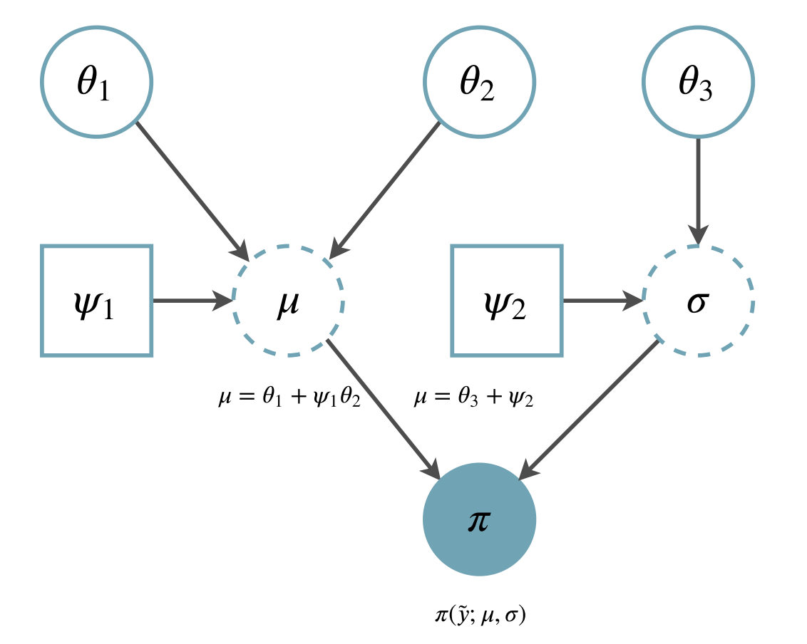
Example of computational graph expressing simple probabilistic model
Problem introduction
Back to geology: How thick is my layer?
Let’s start with the simplest model in structural geology we have been able to come up and trying to be agonizingly pedantic about it. You want to model the thickness of one layer on one specific outcrop and we want to be right. To be sure, we will go during 10 years once per month with a tape measure and we will write down the value on the tape. Finally, 10 years have passed and we are ready to give a conclusive answer. However, out of 120 observations, there are 120 distinct numbers. The first thing we need to reconcile is that any measurements of any phenomenon are isolated. Changes in the environment—maybe some earthquake—or in the way we gather the data—we changed the measurement device or simply our eyes got tired over the years—will also influence which observations \(y\) we end up with. No matter the exact source of the variability, all these processes define the Observation space, \(Y\). Any observational space is going to have some kind of structure that can be modeled for a probability density function called data generating process \(\pi^\dagger\). In other words, there is a latent process—which is a complex combination of several dynamics and limitations—that every time we perform a measurement will yield a value following a certain probability function. Now, to the question what is the thickness of the layer, the answer that better describe the 120 measurements will have to be a probability density function instead of a single value but how can we know what probability function is the right one?
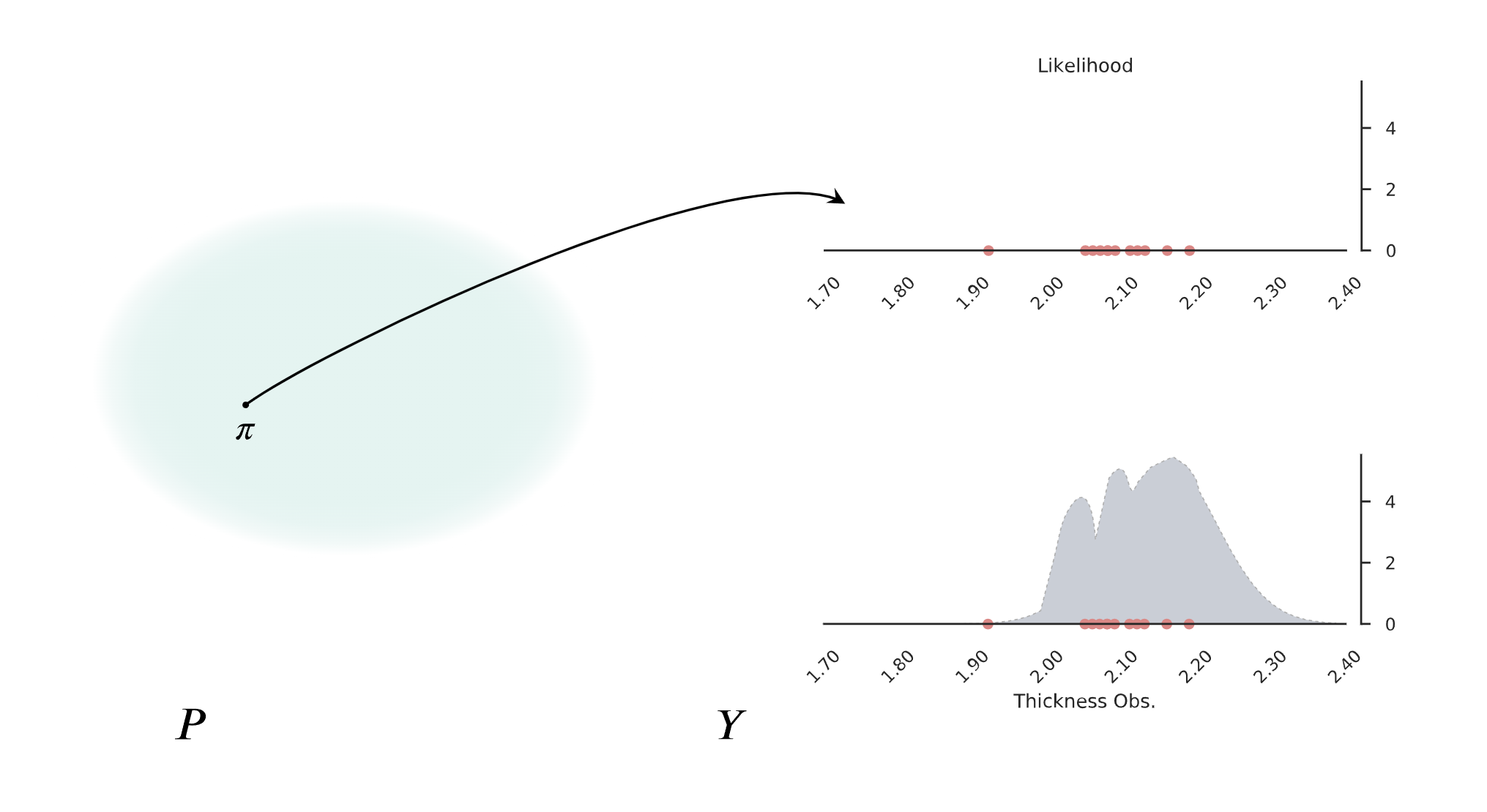
Example of a probability density function fitting to observational data.
The probabilistic model
Note
Add somewhere that \(\theta\) in probabilistic modeling is a random variable and therefore a simplification of saying mean and standard deviation.
The data generating process is latent. Therefore, it will be impossible to perfectly describe it. At this point, we need to compromise and start to make assumptions and choose a model. Any probabilistic family, \(\pi(y;\Theta)\), consist of two distinct sets: observations, \(y\), and model parameters \(\Theta\). Depending on which set is fixed, we obtain either (i) the forward view: for a given set of \(\Theta\) there is a probability of sampling \(y\), or (ii) the inverse view: the observed \(y\) is so much likely for these values of \(\Theta\). Here, we assume that we perform inverse statistics and hence we fix the observations \(y\). For this example, we can assume that the generating process belongs to the Gaussian family:
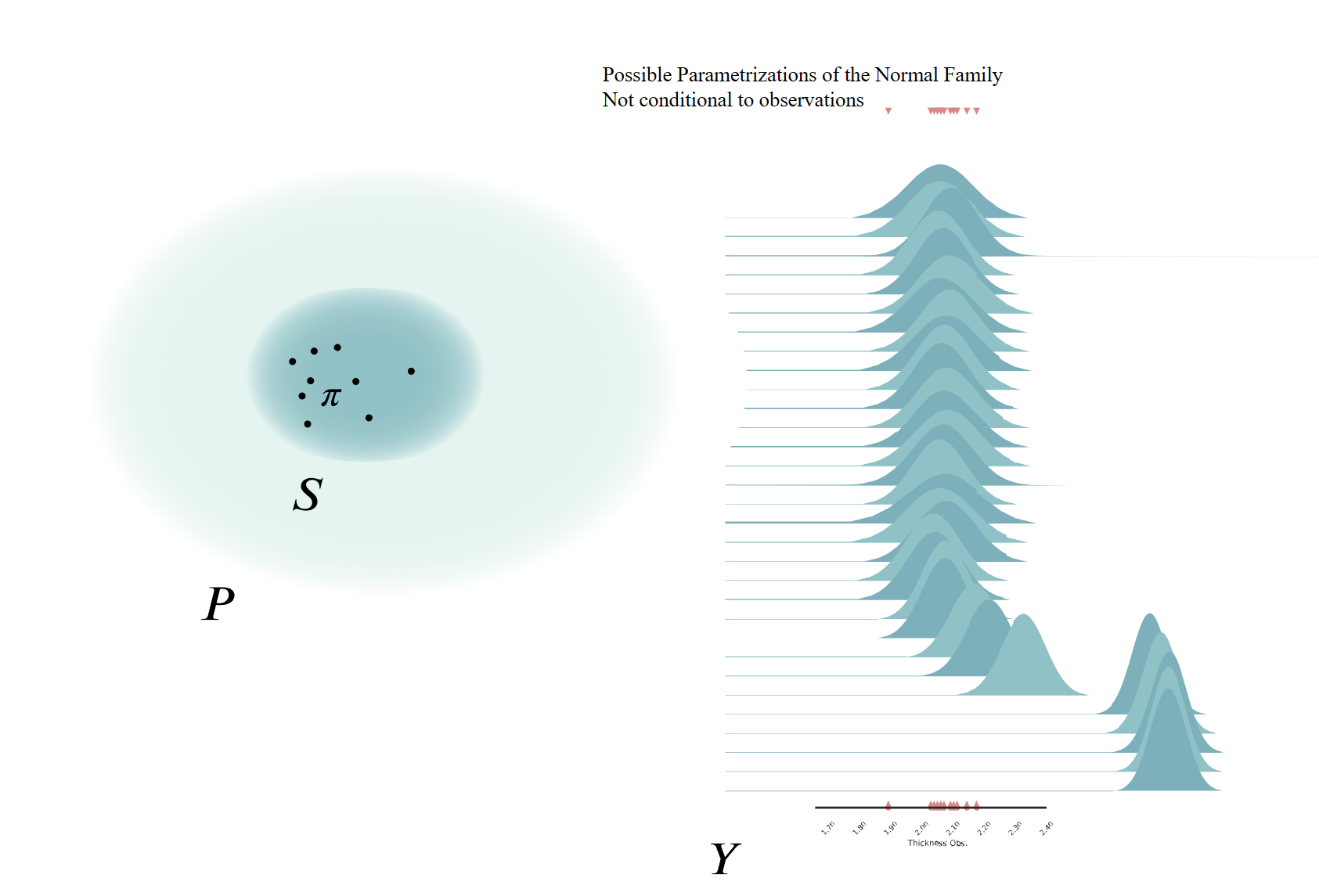
The joy plot has to be random!
No matter which probability density function we choose, for real applications, we will never find the exact data generating process—neither will we be able to say if we have found it for that matter—due to an oversimplification of reality. In Chapter sec:model_selection we will delve into this topic.
Once the model is defined we need to infer the set of parameters \(\Theta\) of the family of density functions over the observational space, \(\pi_S(y;\Theta)\). In the case of the normal family, we need to infer the value of the mean, \(\mu\), and standard deviation, \(\sigma\). Up to this point, all the description of the probabilistic modelling is agnostic in relation to Frequentist or Bayesian views.
Bayesian inference as formalisation of the above
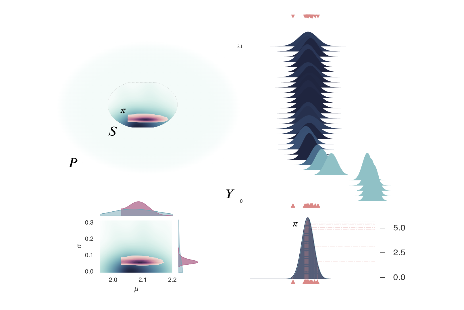
Bayesian inference applied to the problem.
Bayesian inference is based on using the actual observations of reality, \(\tilde{y}\), as conditional probability of a prior definition of \(\Theta\). This construct enables to infer—learn—which model parameters will fit better the observation by “optimising’’ for regions of high-density mass. The simplicity of Bayes equation hides an elegant modular formulation that allows infinite complex trees of conditional probability. However, the dependency of a multidimensional integral has limited its adoption in engineering and other highly complex models. Thankfully, due to the latest advancements in algorithms and computing resources, we are at the dawn of scaling Bayesian networks to a level capable to substantially
License
The code in this case study is copyrighted by Miguel de la Varga and licensed under the new BSD (3-clause) license:
https://opensource.org/licenses/BSD-3-Clause
The text and figures in this case study are copyrighted by Miguel de la Varga and licensed under the CC BY-NC 4.0 license:
https://creativecommons.org/licenses/by-nc/4.0/ Make sure to replace the links with actual hyperlinks if you’re using a platform that supports it (e.g., Markdown or HTML). Otherwise, the plain URLs work fine for plain text.
