2 - Probabilistic Geomodel
Probability density transformation
In the example above the parameters that define the likelihood function \(\pi_S(\theta)\) were directly the prior parameters that we define–the top most level of the probability graph. The simplicity of that model allows for an easy interpretation of the whole inference as the joint probability of the prior distributions, \(\mu_\theta\) and \(\sigma_\theta\), and likelihood functions \(\pi(y|\theta)\) (for one observation). However, there is not reason why the prior random variable—e.g. \(\mu_\theta\) or \(\sigma_\theta\) above—has to derive from one of the “classical” probability density functions—e.g. Normal or Gamma. This means that we can perform as many transformations of a random variables, \(\theta\), as we please before we plug them into a likelihood function, \(\pi(y|\theta)\). This is important because usually we will be able to describe \(\theta\) as function of other random variables either because they are easier to estimate or because it will allow to grow the probabilistic model to integrate multiple data set and knowledge in a coherent fashion.
Probabilistic modelling with GemPy
In structural geology, we want to combine different types of data—i.e. geometrical measurements, geophysics, petrochemical data—usually using as a prevailing model a common earth model. For the sake of simplicity, in this example, we will combine different type of geometric information into one single probabilistic model. Let’s build on the previous idea in order to extend the conceptual case above back to geological modelling.
Lucky for us, after we perform the first inference on the thickness, \(\tilde{y}_{thickness}\) of the model, we find out that a colleague has been gathering data at the exact same outcrop but in his case he was recording the location of the top \(\tilde{y}_{top}\) and bottom \(\tilde{y}_{bottom}\) interfaces of the layer. We can relate the three data sets with simple algebra:
or,
now the question is which probabilistic model design is more suitable. In the end this relates directly to the question the model is trying to answer—and possible limitations on the algorithms used—since joint probability follows the commutative and associative properties.
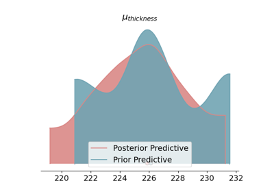
Example of Inference

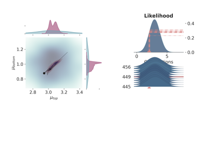
Prior (in blue) and posterior distributions (in red) of all the parameters of the probabilistic model \(\theta\) (the full list of values of the simulation can be found in Appendix X). Case A) correspond to the subtraction equation while Case B) has been generated with the summation equation. Both cases yield the exact same posterior for the random variables—within the Monte Carlo error—as expected.
Correlations
Furthermore, keep in mind that the inference happens in a multidimensional manifold—although for obvious visualization reasons we display each parameter independently. This means that although in the previous figures the posterior distributions seem independent, a closer examination—e.g. joint plots—uncovers correlation in the parameters.
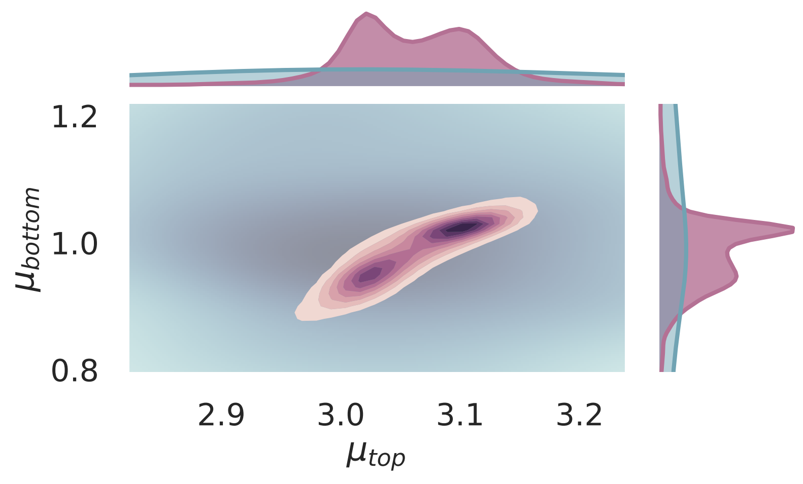
Correlations between parameters can be uncovered with joint plots.
License
The code in this case study is copyrighted by Miguel de la Varga and licensed under the new BSD (3-clause) license:
https://opensource.org/licenses/BSD-3-Clause
The text and figures in this case study are copyrighted by Miguel de la Varga and licensed under the CC BY-NC 4.0 license:
https://creativecommons.org/licenses/by-nc/4.0/ Make sure to replace the links with actual hyperlinks if you’re using a platform that supports it (e.g., Markdown or HTML). Otherwise, the plain URLs work fine for plain text.