1 - First example of inference
Simple example using Pyro: Moving the bell
We can sum up the workflow above in the following steps:
We chose a probabilistic density function family \(\pi\)—e.g., of the Gaussian or uniform families, \(\pi_S(\theta)\) to approximate the data generating process.
We narrow the possible values of \(\theta\)—mean and standard deviation in the case of a Normal distribution—with domain knowledge (notice that although \(\pi_S\) is a subset of \(\pi_P\), its size is infinite and therefore exhaustive approaches are unfeasible).
We use Bayesian inference to condition the prior estimations to our samples of reality \(\pi_S(\tilde{y})|\theta)\).
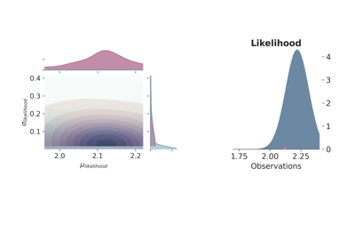
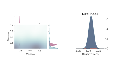
Back to the thickness example, we need to assign some prior distribution to the mean and standard deviation of the thickness; for example, we can take a naive approach and use the values of the crust, or on the contrary, we could use only the data we gathered and maybe one or two references. At this stage, there is not one single valid answer. To analyze how different priors affect, we will use 4 possible configurations, 2 of them using a normal distribution for the mean of a Gaussian likelihood function and the other 2 using a uniform distribution—between 0 and 10 in order to keep it as uninformative as possible while still giving valid physical values:
Normal |
Uniform |
|---|---|
\(\theta_\mu \sim \mathcal{N}(\mu=2.08, \sigma=0.07)\) |
\(\theta_\mu \sim \mathcal{U}(a=0, b=10)\) |
\(\theta_\sigma \sim \Gamma(\alpha=0.3, \beta=3)\) |
\(\theta_\sigma \sim \Gamma(=1.0, \beta=0.7)\) |
\(\pi_S(y|\theta) \sim \mathcal{N}(\mu=\theta_\mu, \sigma=\theta_\sigma)\) |
\(\pi_S(y|\theta) \sim \mathcal{N}(\mu=\theta_\mu, \sigma=\theta_\sigma)\) |
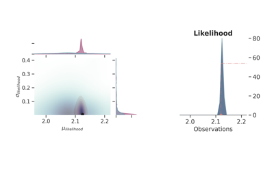
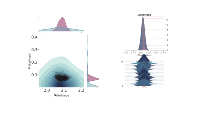
The standard deviation is in both cases a quite uninformative Gamma distribution. Besides using different probability functions to describe one of the model parameters, we have also repeated the same simulation either using one observation, \(\tilde{y}\) at 2.12 m, or 10 observation spread randomly (as random as a human possibly can) around 2.10. Figure fig-models1 shows the joint prior (in blue) and posterior (in red) distributions for the 4 probabilistic models, as well as, the maximum likelihood function.
Result description and some words about uninformative prior
The first thing that comes to mind by looking at the results is that the model choice has a clear impact on the final result although the more observations are included the more similar both models get indistinctively of the priors. Therefore, it is interesting to compare the two cases with just one observation (Figure fig-models1, above), curiously enough, the probabilistic model with the normal distribution underrepresents the model uncertainty—assuming that the simulations c) and d) are closer to the real data generating process—while the uniform clearly portrays too much variance. Once again, considering that the only window to the data generating model are indirect observation of a phenomenon, in regimes of low and/or noisy data points there is only so much information we can extract from the data. This is to say that there are not truly uninformative prior distributions—although there are theoretical limits such as maximum entropy—and therefore the best we can do is to use the knowledge of the practitioner as first educated guess.
Type of probabilistic models
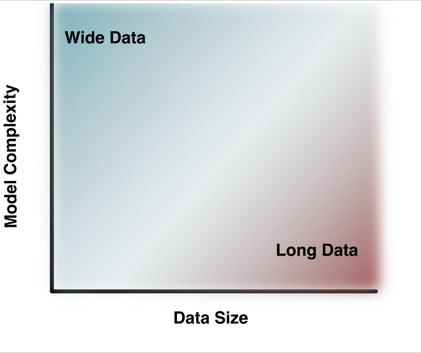
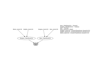
Example of computational graph expressing simple probabilistic model :name: fig-model-type
Depending on the type of phenomenon analyzed and the model complexity, two different categories of problems emerge: Wide data and Long data. Long data problems are characterized by a large number of repetitions of the same phenomenon, allowing all sorts of machine learning and big data approaches. Wide data, on the other hand, features few repetitions of several phenomena that rely on complex mathematical models to relate them [1]. Structural geology is an unequivocal example of the second case due to the sheer size and scale it is aimed to be modeled. For this reason, a systematic way to include domain knowledge into the system via informative prior distributions becomes a powerful tool in the endeavor of integrating as much information as possible in a single mathematical model.
Priors as joint probability
In low data regimes where domain knowledge plays such an essential role, it is crucial to include as much coherent information as possible. Simply giving the best estimate of the data generating function may work for simple systems where our brains are capable to relate available data and knowledge. Nevertheless, as complexity rises, a more systematic way of combining data and knowledge becomes fundamental. Models are in essence a tool to generate best guesses following mathematical axioms. This view of models as tools to combine different sources of data and knowledge to help to define the best guess of a latent data generating process may seem an unnecessary convoluted way to explain Bayesian statistics. However, in our opinion, this view helps to change the perspective of prior distributions—from terms of “belief” as a source of bias—to a more general perspective of using joint probability as a means to combine complex mathematical models and observations in a mathematically sound and transparent manner.
License
The code in this case study is copyrighted by Miguel de la Varga and licensed under the new BSD (3-clause) license:
https://opensource.org/licenses/BSD-3-Clause
The text and figures in this case study are copyrighted by Miguel de la Varga and licensed under the CC BY-NC 4.0 license:
https://creativecommons.org/licenses/by-nc/4.0/ Make sure to replace the links with actual hyperlinks if you’re using a platform that supports it (e.g., Markdown or HTML). Otherwise, the plain URLs work fine for plain text.