Normal Prior, several observations

# We previously mentioned that we can optimize this model to better fit observations.

For this, we generate a prior from the model we previously created, the one with multiple observations from y_obs_list.

# In the following, samples are iteratively drawn and evaluated to form the posterior. This generates what is called a “trace”. A predictive Posterior distribution is then generated from said trace.

# sphinx_gallery_thumbnail_number = -1

import arviz as az
import matplotlib.pyplot as plt
import pyro
import torch
from matplotlib.ticker import StrMethodFormatter

from gempy_probability.plot_posterior import PlotPosterior
from _aux_func import infer_model
az.style.use("arviz-doc")

# Sample observations
y_obs_list = torch.tensor([2.12, 2.06, 2.08, 2.05, 2.08, 2.09,
                           2.19, 2.07, 2.16, 2.11, 2.13, 1.92])
pyro.set_rng_seed(4003)

# Infer model from the observations
az_data = infer_model(
    distributions_family="normal_distribution",
    data=y_obs_list
)

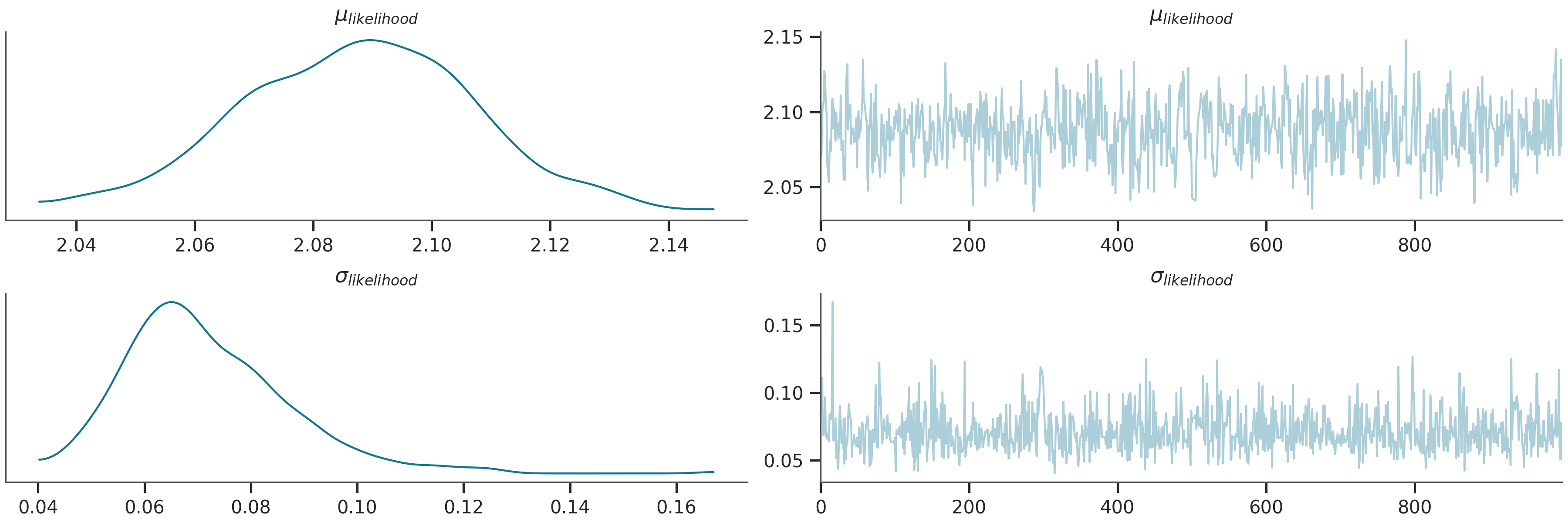
# Plot the trace of the inference process
az.plot_trace(az_data)
plt.show()

Warmup:   0%|          | 0/1100 [00:00, ?it/s]
Warmup:   0%|          | 1/1100 [00:00,  2.36it/s, step size=1.80e+00, acc. prob=1.000]
Warmup:   2%|▏         | 27/1100 [00:00, 65.10it/s, step size=3.15e-02, acc. prob=0.751]
Warmup:   4%|▍         | 48/1100 [00:00, 101.13it/s, step size=2.64e-02, acc. prob=0.766]
Warmup:   6%|▌         | 65/1100 [00:00, 118.49it/s, step size=3.79e-02, acc. prob=0.775]
Warmup:   7%|▋         | 82/1100 [00:00, 131.80it/s, step size=1.89e-02, acc. prob=0.774]
Warmup:   9%|▉         | 101/1100 [00:00, 147.83it/s, step size=4.21e-01, acc. prob=0.760]
Sample:  14%|█▎        | 149/1100 [00:01, 240.53it/s, step size=4.21e-01, acc. prob=0.826]
Sample:  17%|█▋        | 191/1100 [00:01, 291.49it/s, step size=4.21e-01, acc. prob=0.835]
Sample:  22%|██▏       | 240/1100 [00:01, 347.90it/s, step size=4.21e-01, acc. prob=0.830]
Sample:  26%|██▌       | 283/1100 [00:01, 371.06it/s, step size=4.21e-01, acc. prob=0.823]
Sample:  30%|██▉       | 327/1100 [00:01, 389.20it/s, step size=4.21e-01, acc. prob=0.826]
Sample:  34%|███▍      | 376/1100 [00:01, 418.81it/s, step size=4.21e-01, acc. prob=0.830]
Sample:  39%|███▉      | 427/1100 [00:01, 445.19it/s, step size=4.21e-01, acc. prob=0.831]
Sample:  43%|████▎     | 473/1100 [00:01, 437.79it/s, step size=4.21e-01, acc. prob=0.830]
Sample:  47%|████▋     | 521/1100 [00:01, 449.11it/s, step size=4.21e-01, acc. prob=0.827]
Sample:  52%|█████▏    | 567/1100 [00:01, 442.12it/s, step size=4.21e-01, acc. prob=0.821]
Sample:  56%|█████▌    | 617/1100 [00:02, 451.88it/s, step size=4.21e-01, acc. prob=0.815]
Sample:  60%|██████    | 664/1100 [00:02, 455.83it/s, step size=4.21e-01, acc. prob=0.815]
Sample:  65%|██████▍   | 710/1100 [00:02, 445.61it/s, step size=4.21e-01, acc. prob=0.816]
Sample:  69%|██████▉   | 757/1100 [00:02, 447.53it/s, step size=4.21e-01, acc. prob=0.818]
Sample:  73%|███████▎  | 802/1100 [00:02, 434.88it/s, step size=4.21e-01, acc. prob=0.822]
Sample:  77%|███████▋  | 846/1100 [00:02, 427.99it/s, step size=4.21e-01, acc. prob=0.820]
Sample:  82%|████████▏ | 899/1100 [00:02, 455.67it/s, step size=4.21e-01, acc. prob=0.819]
Sample:  86%|████████▌ | 945/1100 [00:02, 438.46it/s, step size=4.21e-01, acc. prob=0.818]
Sample:  90%|█████████ | 991/1100 [00:02, 441.91it/s, step size=4.21e-01, acc. prob=0.819]
Sample:  95%|█████████▍| 1043/1100 [00:03, 462.72it/s, step size=4.21e-01, acc. prob=0.818]
Sample:  99%|█████████▉| 1090/1100 [00:03, 463.32it/s, step size=4.21e-01, acc. prob=0.820]
Sample: 100%|██████████| 1100/1100 [00:03, 348.14it/s, step size=4.21e-01, acc. prob=0.820]

/home/leguark/.virtualenvs/gempy_dependencies/lib/python3.10/site-packages/arviz/data/io_pyro.py:158: UserWarning: Could not get vectorized trace, log_likelihood group will be omitted. Check your model vectorization or set log_likelihood=False
  warnings.warn(
posterior predictive shape not compatible with number of chains and draws.This can mean that some draws or even whole chains are not represented.

Raw observations

The behavior of this chain is controlled by the observations we fed into the model. Let’s have a look at the observations and how they are distributed:

p = PlotPosterior(az_data)
p.create_figure(figsize=(9, 3), joyplot=False, marginal=False)
p.plot_normal_likelihood(
    mean='$\\mu_{likelihood}$',
    std='$\\sigma_{likelihood}$',
    obs='$y$',
    iteration=-1,
    hide_bell=True
)
p.likelihood_axes.set_xlim(1.90, 2.2)
p.likelihood_axes.xaxis.set_major_formatter(StrMethodFormatter('{x:,.2f}'))
for tick in p.likelihood_axes.get_xticklabels():
    tick.set_rotation(45)
plt.show()

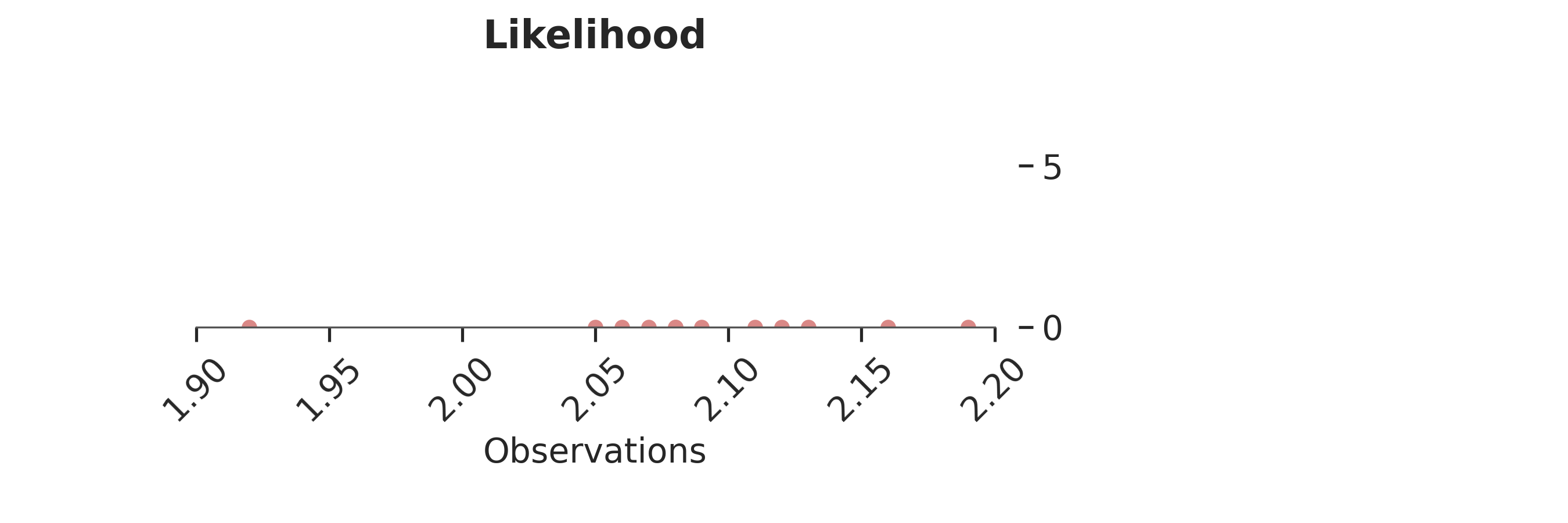
The bulk of observations is between 2.05 and 2.15, with one outlier at 1.92.

Final inference

Let’s now plot the inferred posterior distribution (i.e., the last sample iteration) and the observations:

p = PlotPosterior(az_data)
p.create_figure(figsize=(9, 3), joyplot=False, marginal=False)
p.plot_normal_likelihood(
    mean='$\\mu_{likelihood}$',
    std='$\\sigma_{likelihood}$',
    obs='$y$',
    iteration=-1,
    hide_bell=False
)
p.likelihood_axes.set_xlim(1.70, 2.40)
p.likelihood_axes.xaxis.set_major_formatter(StrMethodFormatter('{x:,.2f}'))
for tick in p.likelihood_axes.get_xticklabels():
    tick.set_rotation(45)
plt.show()

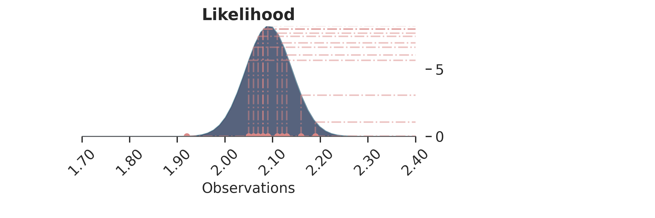
The bell-peak is centered on a cluster of observations, but the outlier at 1.92 shifts the distribution slightly. Joyplot ——- To visualize the change in distribution across iterations, we use a joyplot. This allows us to see how the mean ($\mu$) and standard deviation ($\sigma$) change over time with progressive sampling:

p = PlotPosterior(az_data)
p.create_figure(figsize=(9, 9), joyplot=True, marginal=False, likelihood=False, n_samples=31)
p.plot_joy(
    var_names=('$\\mu_{likelihood}$', '$\\sigma_{likelihood}$'),
    obs='$y$',
    iteration=14
)
plt.show()

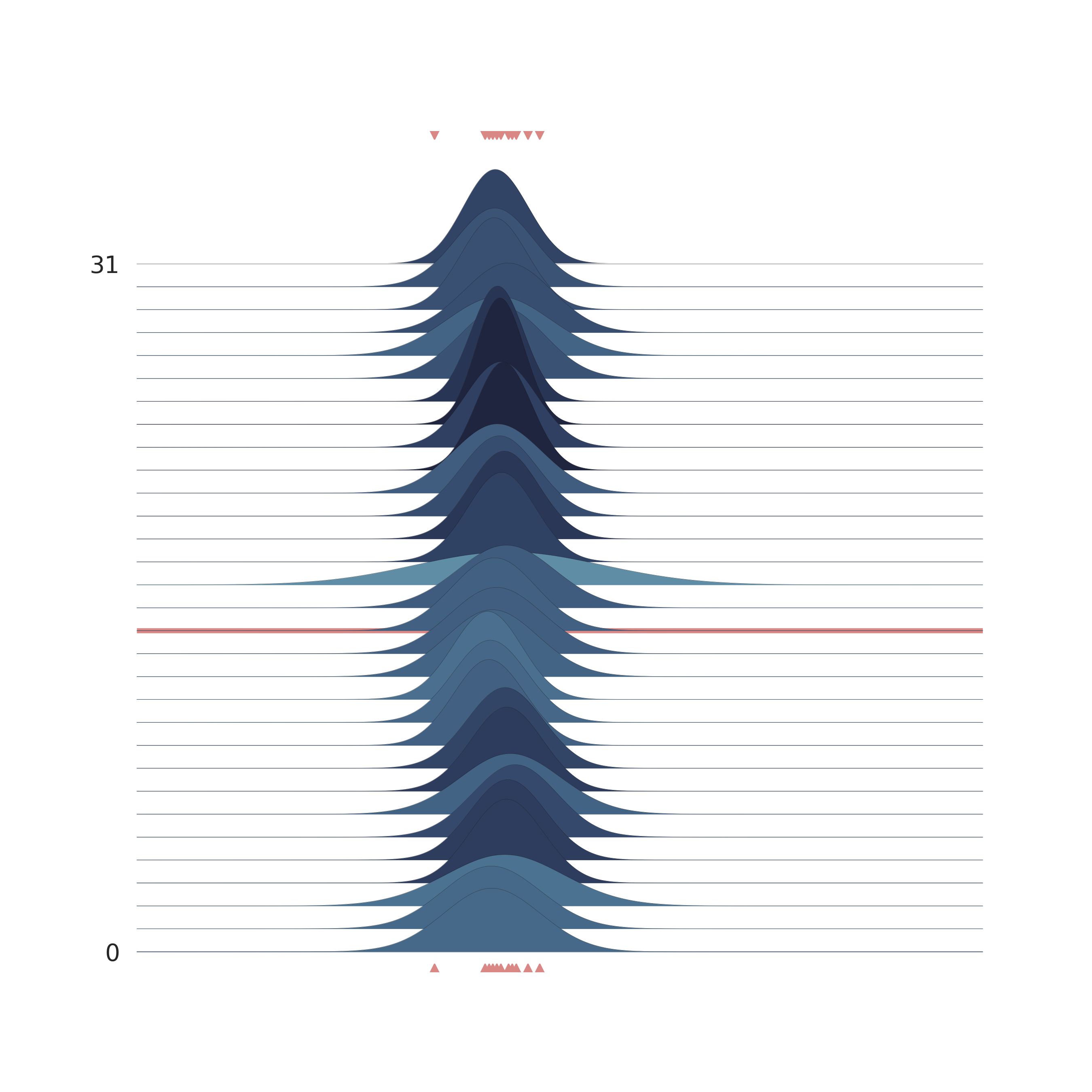
The following animation shows how the distribution evolves during sampling. Darker colors represent an increase in likelihood as the Markov Chain explores the probability space.

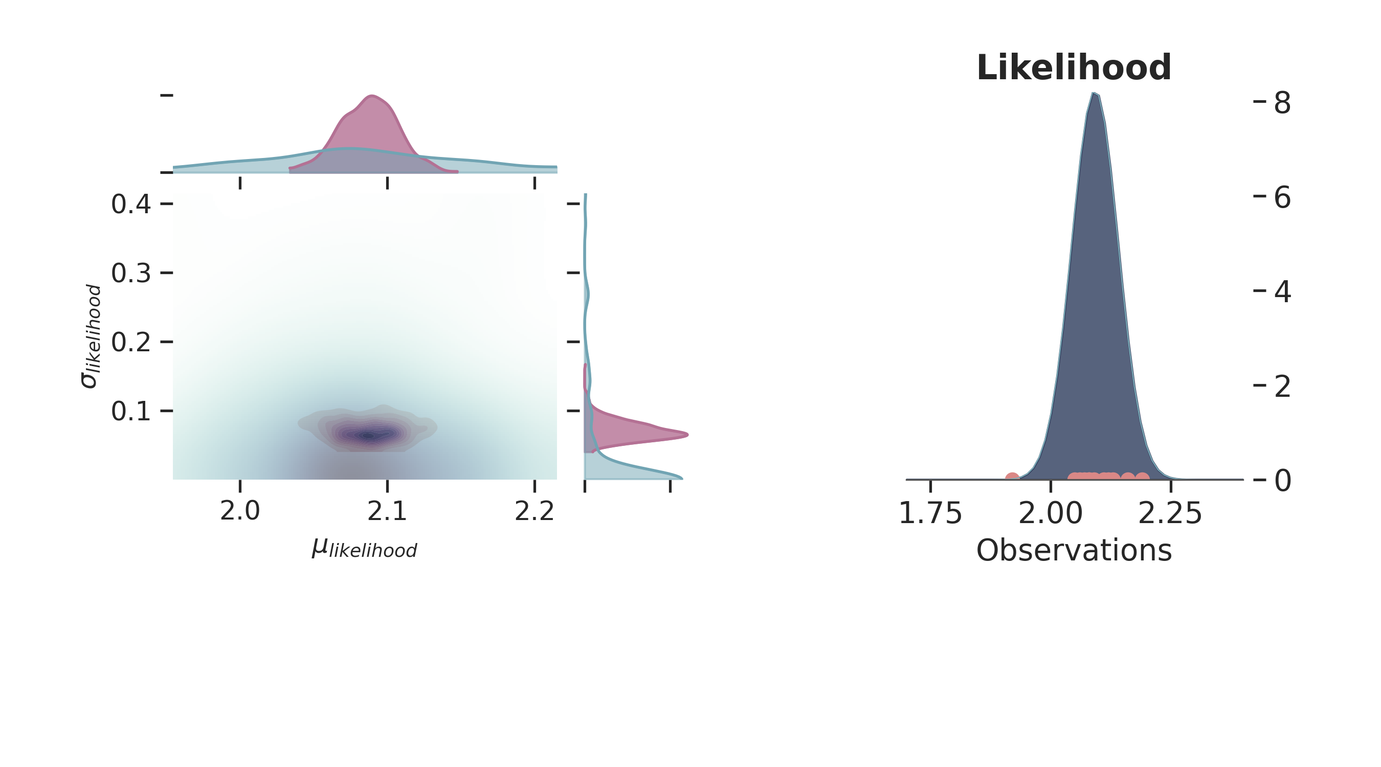
Joint Probability

p = PlotPosterior(az_data)
p.create_figure(figsize=(9, 5), joyplot=False, marginal=True, likelihood=True)
p.plot_marginal(
    var_names=['$\\mu_{likelihood}$', '$\\sigma_{likelihood}$'],
    plot_trace=False,
    credible_interval=0.95,
    kind='kde',
    joint_kwargs={'contour': True, 'pcolormesh_kwargs': {}},
    joint_kwargs_prior={'contour': False, 'pcolormesh_kwargs': {}}
)
p.plot_normal_likelihood(
    mean='$\\mu_{likelihood}$',
    std='$\\sigma_{likelihood}$',
    obs='$y$',
    iteration=-1,
    hide_lines=True
)
p.likelihood_axes.set_xlim(1.70, 2.40)
plt.show()

Sampling Process

Below is a gif of the first 100 samples, starting from the 10th iteration:

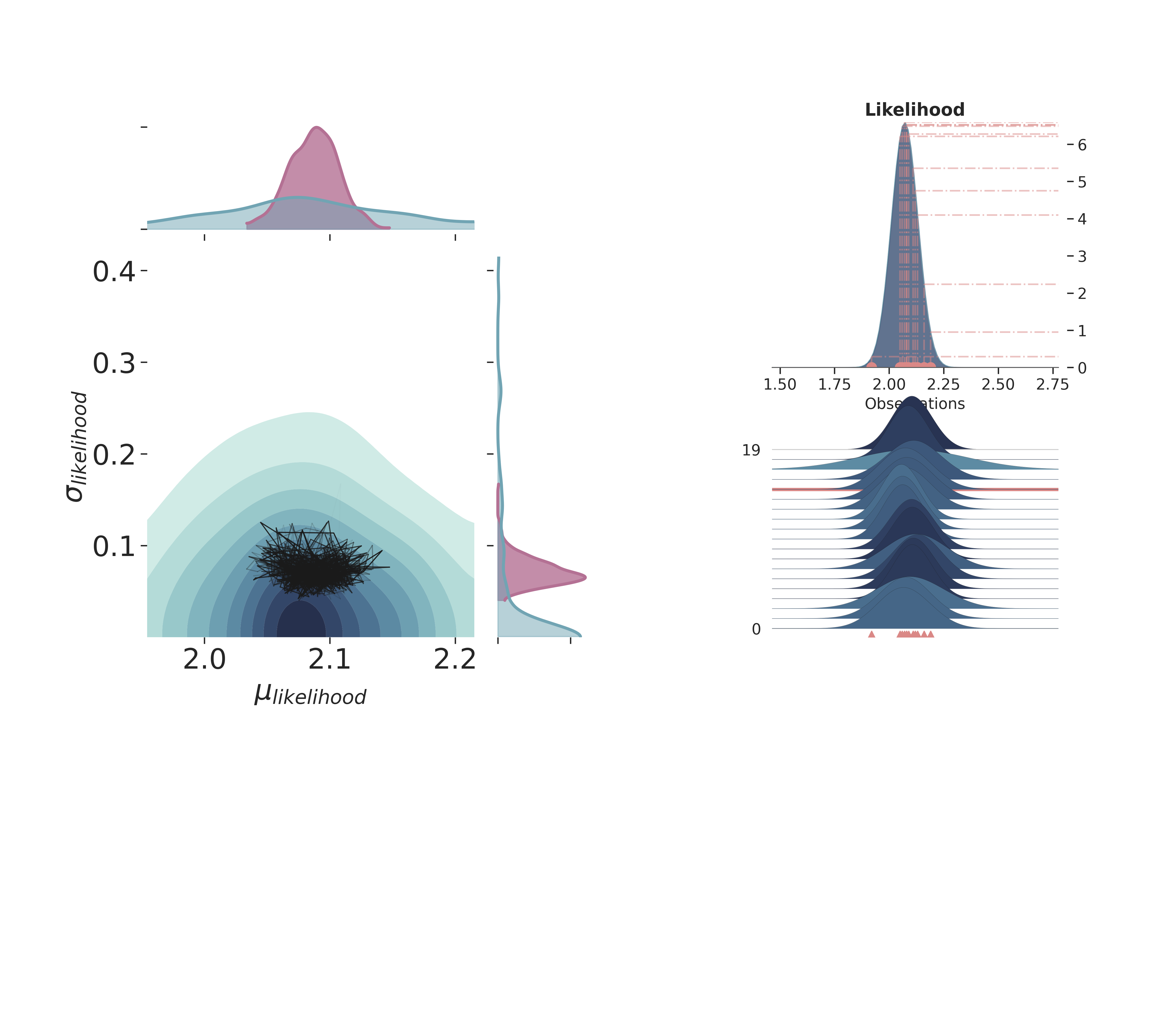
Full Plot

p3 = PlotPosterior(az_data)
p3.create_figure(figsize=(15, 13), joyplot=True, marginal=True, likelihood=True, n_samples=19)
p3.plot_posterior(
    prior_var=['$\\mu_{likelihood}$', '$\\sigma_{likelihood}$'],
    like_var=['$\\mu_{likelihood}$', '$\\sigma_{likelihood}$'],
    obs='$y$',
    iteration=-5,
    marginal_kwargs={
            'plot_trace'       : True,
            'credible_interval': .95,
            'kind'             : 'kde',
            "joint_kwargs"     : {
                    'contour'          : True,
                    'pcolormesh_kwargs': {}
            },
    }
)
plt.show()

/home/leguark/gempy_probability/gempy_probability/plot_posterior.py:254: UserWarning: color is redundantly defined by the 'color' keyword argument and the fmt string "bo" (-> color='b'). The keyword argument will take precedence.
  self.axjoin.plot(theta1_val, theta2_val, 'bo', ms=6, color='k')

License

The code in this case study is copyrighted by Miguel de la Varga and licensed under the new BSD (3-clause) license:

https://opensource.org/licenses/BSD-3-Clause

The text and figures in this case study are copyrighted by Miguel de la Varga and licensed under the CC BY-NC 4.0 license:

https://creativecommons.org/licenses/by-nc/4.0/ Make sure to replace the links with actual hyperlinks if you’re using a platform that supports it (e.g., Markdown or HTML). Otherwise, the plain URLs work fine for plain text.