Uniform Prior, several observations

# sphinx_gallery_thumbnail_number = -1

import arviz as az
import matplotlib.pyplot as plt
import pyro
import torch
from matplotlib.ticker import StrMethodFormatter

from gempy_probability.plot_posterior import PlotPosterior

from _aux_func import infer_model

az.style.use("arviz-doc")

y_obs = torch.tensor([2.12])
y_obs_list = torch.tensor([2.12, 2.06, 2.08, 2.05, 2.08, 2.09,
                           2.19, 2.07, 2.16, 2.11, 2.13, 1.92])
pyro.set_rng_seed(4003)

az_data = infer_model(
    distributions_family="uniform_distribution",
    data=y_obs_list
)
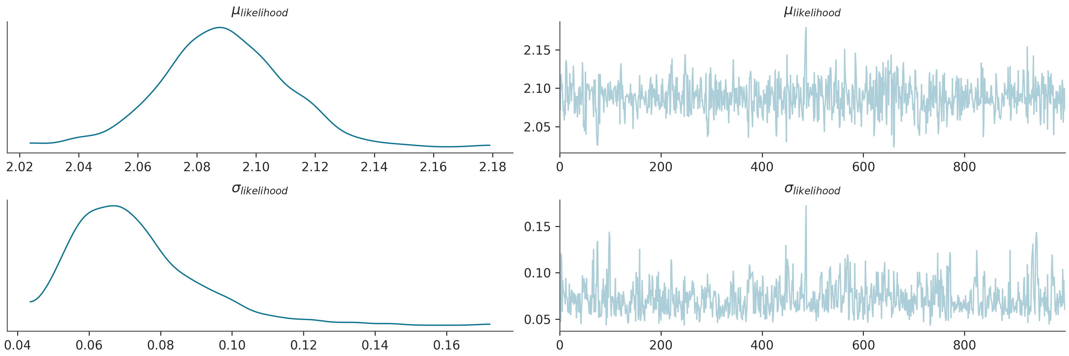
az.plot_trace(az_data)
plt.show()

Warmup:   0%|          | 0/1100 [00:00, ?it/s]
Warmup:   2%|▏         | 18/1100 [00:00, 173.83it/s, step size=5.45e-02, acc. prob=0.730]
Warmup:   3%|▎         | 36/1100 [00:00, 133.48it/s, step size=2.70e-02, acc. prob=0.752]
Warmup:   5%|▍         | 50/1100 [00:00, 98.13it/s, step size=1.36e-02, acc. prob=0.756]
Warmup:   6%|▌         | 64/1100 [00:00, 108.23it/s, step size=3.37e-02, acc. prob=0.769]
Warmup:   7%|▋         | 79/1100 [00:00, 117.67it/s, step size=1.28e-02, acc. prob=0.767]
Warmup:   8%|▊         | 92/1100 [00:00, 101.23it/s, step size=2.50e-01, acc. prob=0.756]
Sample:  11%|█         | 119/1100 [00:00, 143.45it/s, step size=5.24e-01, acc. prob=0.943]
Sample:  14%|█▎        | 150/1100 [00:01, 186.81it/s, step size=5.24e-01, acc. prob=0.935]
Sample:  16%|█▋        | 179/1100 [00:01, 214.69it/s, step size=5.24e-01, acc. prob=0.942]
Sample:  19%|█▉        | 212/1100 [00:01, 245.65it/s, step size=5.24e-01, acc. prob=0.946]
Sample:  22%|██▏       | 247/1100 [00:01, 273.55it/s, step size=5.24e-01, acc. prob=0.941]
Sample:  26%|██▌       | 281/1100 [00:01, 289.86it/s, step size=5.24e-01, acc. prob=0.943]
Sample:  28%|██▊       | 311/1100 [00:01, 292.67it/s, step size=5.24e-01, acc. prob=0.944]
Sample:  31%|███       | 343/1100 [00:01, 300.30it/s, step size=5.24e-01, acc. prob=0.944]
Sample:  34%|███▍      | 375/1100 [00:01, 302.36it/s, step size=5.24e-01, acc. prob=0.945]
Sample:  37%|███▋      | 406/1100 [00:01, 302.12it/s, step size=5.24e-01, acc. prob=0.946]
Sample:  40%|████      | 440/1100 [00:01, 312.59it/s, step size=5.24e-01, acc. prob=0.945]
Sample:  43%|████▎     | 472/1100 [00:02, 310.92it/s, step size=5.24e-01, acc. prob=0.941]
Sample:  46%|████▌     | 504/1100 [00:02, 306.80it/s, step size=5.24e-01, acc. prob=0.942]
Sample:  49%|████▊     | 535/1100 [00:02, 307.44it/s, step size=5.24e-01, acc. prob=0.942]
Sample:  52%|█████▏    | 568/1100 [00:02, 312.35it/s, step size=5.24e-01, acc. prob=0.943]
Sample:  55%|█████▍    | 600/1100 [00:02, 309.31it/s, step size=5.24e-01, acc. prob=0.944]
Sample:  58%|█████▊    | 634/1100 [00:02, 316.60it/s, step size=5.24e-01, acc. prob=0.943]
Sample:  61%|██████    | 666/1100 [00:02, 310.03it/s, step size=5.24e-01, acc. prob=0.943]
Sample:  64%|██████▍   | 704/1100 [00:02, 327.01it/s, step size=5.24e-01, acc. prob=0.942]
Sample:  67%|██████▋   | 738/1100 [00:02, 327.26it/s, step size=5.24e-01, acc. prob=0.942]
Sample:  70%|███████   | 771/1100 [00:03, 323.77it/s, step size=5.24e-01, acc. prob=0.941]
Sample:  73%|███████▎  | 804/1100 [00:03, 312.04it/s, step size=5.24e-01, acc. prob=0.941]
Sample:  76%|███████▋  | 841/1100 [00:03, 327.16it/s, step size=5.24e-01, acc. prob=0.941]
Sample:  80%|███████▉  | 875/1100 [00:03, 329.28it/s, step size=5.24e-01, acc. prob=0.940]
Sample:  83%|████████▎ | 909/1100 [00:03, 320.35it/s, step size=5.24e-01, acc. prob=0.941]
Sample:  86%|████████▌ | 946/1100 [00:03, 334.05it/s, step size=5.24e-01, acc. prob=0.941]
Sample:  89%|████████▉ | 980/1100 [00:03, 320.46it/s, step size=5.24e-01, acc. prob=0.941]
Sample:  92%|█████████▏| 1013/1100 [00:03, 315.45it/s, step size=5.24e-01, acc. prob=0.941]
Sample:  95%|█████████▌| 1045/1100 [00:03, 309.99it/s, step size=5.24e-01, acc. prob=0.941]
Sample:  98%|█████████▊| 1077/1100 [00:03, 306.90it/s, step size=5.24e-01, acc. prob=0.941]
Sample: 100%|██████████| 1100/1100 [00:04, 271.43it/s, step size=5.24e-01, acc. prob=0.941]

/home/leguark/.virtualenvs/gempy_dependencies/lib/python3.10/site-packages/arviz/data/io_pyro.py:158: UserWarning: Could not get vectorized trace, log_likelihood group will be omitted. Check your model vectorization or set log_likelihood=False
  warnings.warn(
posterior predictive shape not compatible with number of chains and draws.This can mean that some draws or even whole chains are not represented.

p = PlotPosterior(az_data)
p.create_figure(figsize=(9, 3), joyplot=False, marginal=False)
p.plot_normal_likelihood(
    mean='$\\mu_{likelihood}$',
    std='$\\sigma_{likelihood}$',
    obs= '$y$',
    iteration=-1,
    hide_bell=True
)
p.likelihood_axes.set_xlim(1.90, 2.2)
p.likelihood_axes.xaxis.set_major_formatter(StrMethodFormatter('{x:,.2f}'))
for tick in p.likelihood_axes.get_xticklabels():
    tick.set_rotation(45)
plt.show()

No matter which probability density function we choose, for real applications we will never find the exact data generated process—neither we will be able to say if we have found it for that matter—due to an oversimplification of reality. For most applications, the usual families of probability density functions and transformations of those are more than enough approximations for the purpose of the model. In Chapter [sec:model_selection], we will delve into this topic.

Once the model is defined we need to infer the set of parameters ( varTheta ) of the family of density functions over the observational space, ( pi_S(y;varTheta) ). In the case of the normal family, we need to infer the value of the mean, ( mu ) and standard deviation ( sigma ). Up to this point, all the description of the probabilistic modelling is agnostic in relation to Frequentist or Bayesian views. These two methodologies diverge on how they infer ( varTheta ).

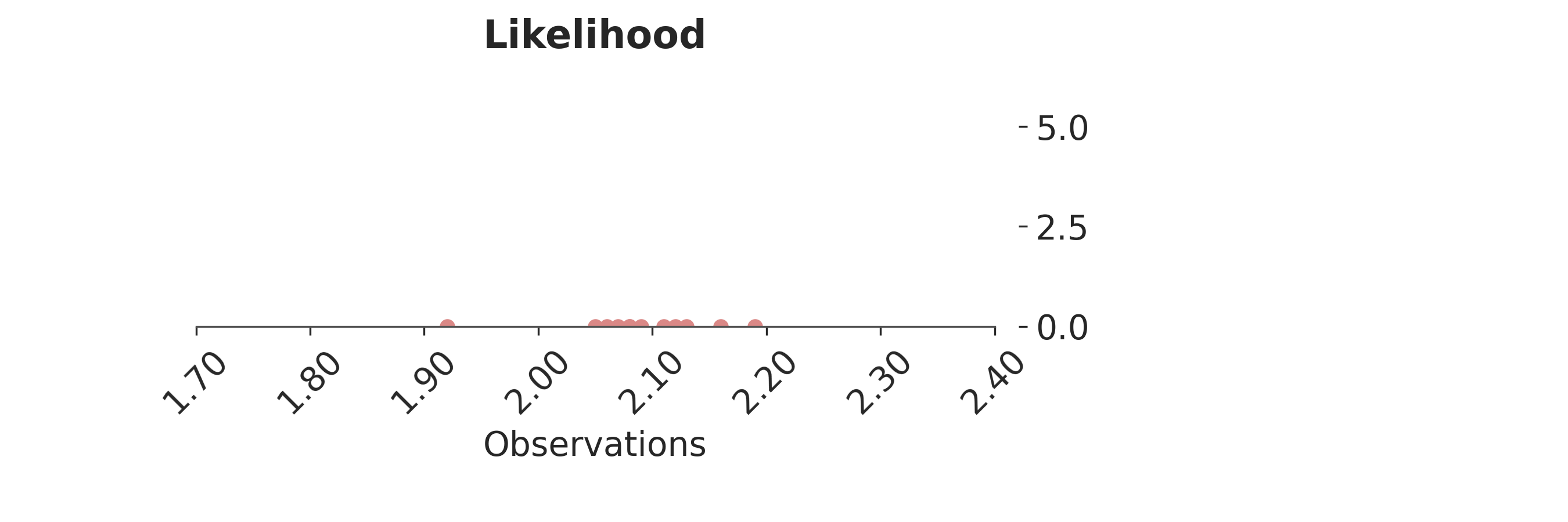
p = PlotPosterior(az_data)
p.create_figure(figsize=(9, 3), joyplot=False, marginal=False)
p.plot_normal_likelihood(
    mean='$\\mu_{likelihood}$',
    std='$\\sigma_{likelihood}$',
    obs= '$y$',
    iteration=-1,
    hide_bell=True
)
p.likelihood_axes.set_xlim(1.70, 2.40)
p.likelihood_axes.xaxis.set_major_formatter(StrMethodFormatter('{x:,.2f}'))
for tick in p.likelihood_axes.get_xticklabels():
    tick.set_rotation(45)
plt.show()

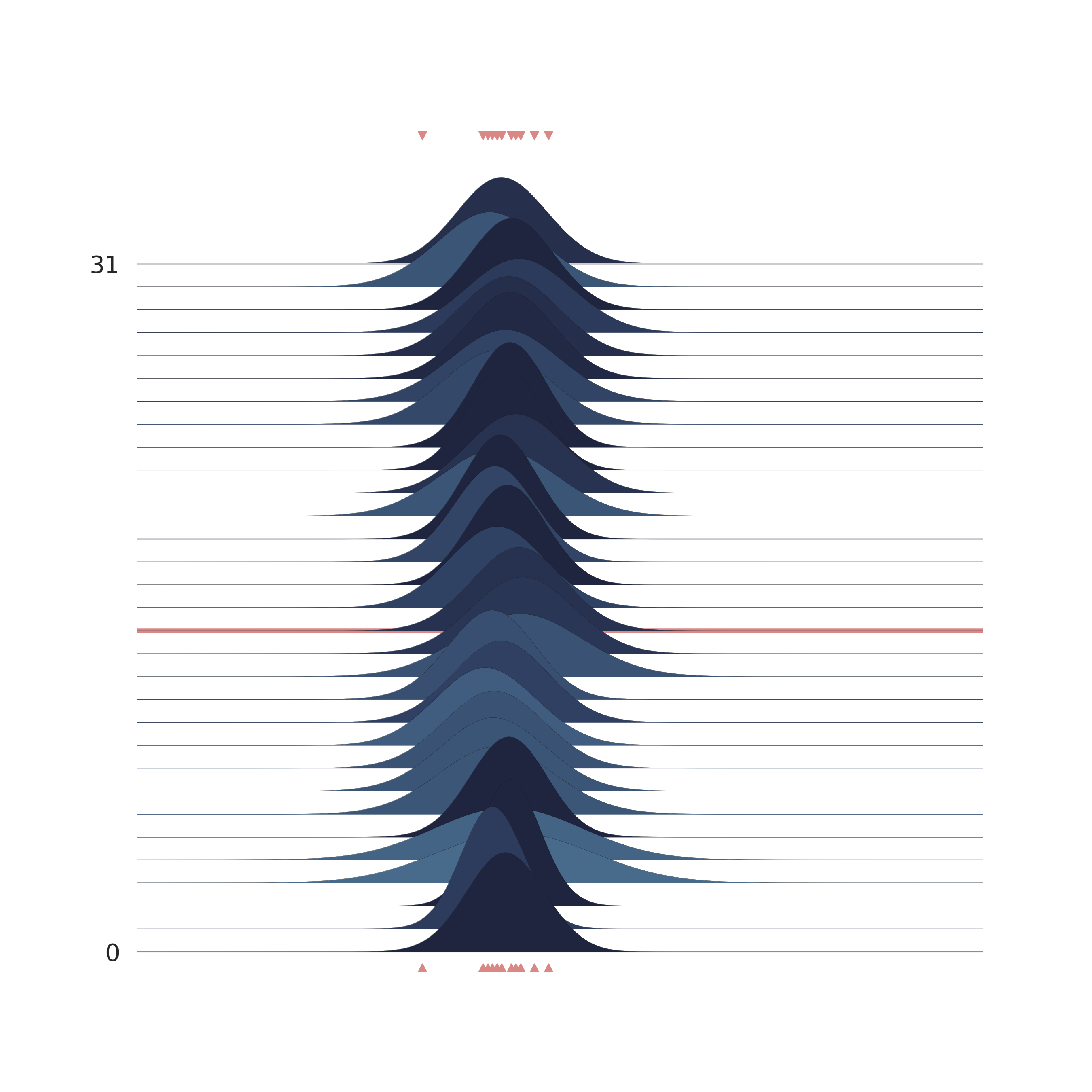
p = PlotPosterior(az_data)

p.create_figure(figsize=(9, 9), joyplot=True, marginal=False, likelihood=False, n_samples=31)
p.plot_joy(
    var_names=('$\\mu_{likelihood}$', '$\\sigma_{likelihood}$'),
    obs='$y$',
    iteration=14
)
plt.show()

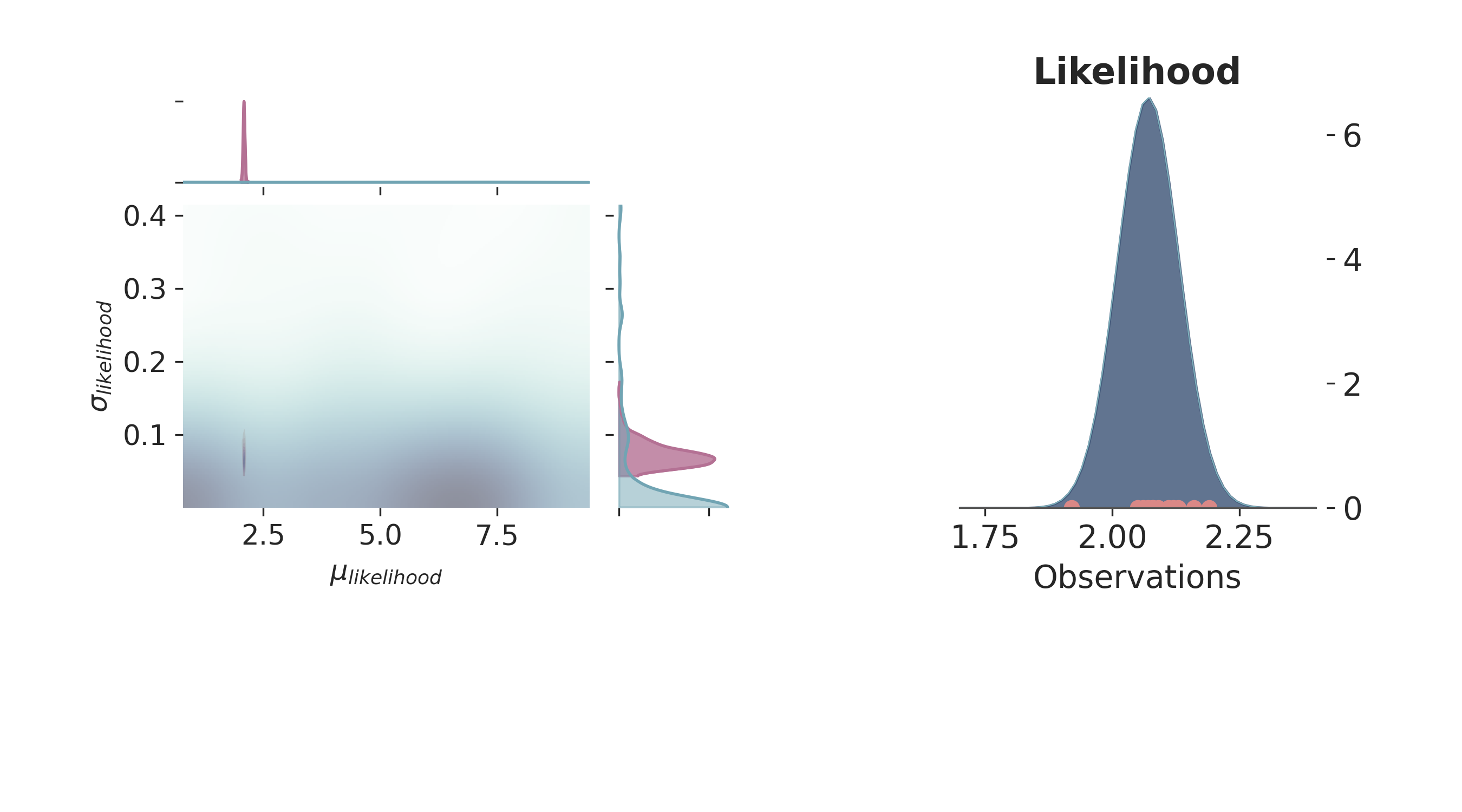
p = PlotPosterior(az_data)

p.create_figure(figsize=(9, 5), joyplot=False, marginal=True, likelihood=True)
p.plot_marginal(
    var_names=['$\\mu_{likelihood}$', '$\\sigma_{likelihood}$'],
    plot_trace=False,
    credible_interval=1,
    kind='kde',
    joint_kwargs={'contour': True, 'pcolormesh_kwargs': {}},
    joint_kwargs_prior={'contour': False, 'pcolormesh_kwargs': {}}
)


p.plot_normal_likelihood(
    mean='$\\mu_{likelihood}$',
    std='$\\sigma_{likelihood}$',
    obs='$y$',
    iteration=-1,
    hide_lines=True
)
p.likelihood_axes.set_xlim(1.70, 2.40)
plt.show()

License

The code in this case study is copyrighted by Miguel de la Varga and licensed under the new BSD (3-clause) license:

https://opensource.org/licenses/BSD-3-Clause

The text and figures in this case study are copyrighted by Miguel de la Varga and licensed under the CC BY-NC 4.0 license:

https://creativecommons.org/licenses/by-nc/4.0/ Make sure to replace the links with actual hyperlinks if you’re using a platform that supports it (e.g., Markdown or HTML). Otherwise, the plain URLs work fine for plain text.