Uniform Prior, single observation

# sphinx_gallery_thumbnail_number = -1
import arviz as az
import matplotlib.pyplot as plt
import pyro
import torch
from matplotlib.ticker import StrMethodFormatter

from gempy_probability.plot_posterior import PlotPosterior
from _aux_func import infer_model

y_obs = torch.tensor([2.12])
y_obs_list = torch.tensor([2.12, 2.06, 2.08, 2.05, 2.08, 2.09,
                           2.19, 2.07, 2.16, 2.11, 2.13, 1.92])
pyro.set_rng_seed(4003)

az_data = infer_model(
    distributions_family="uniform_distribution",
    data=y_obs
)
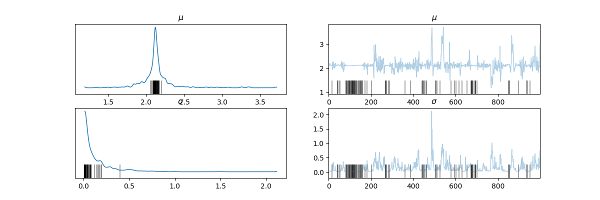
az.plot_trace(az_data)
plt.show()

Warmup:   0%|                                                       | 0/1100 [00:00, ?it/s]
Warmup:   2%|▏           | 17/1100 [00:00, 169.94it/s, step size=1.52e-01, acc. prob=0.746]
Warmup:   3%|▍           | 38/1100 [00:00, 191.85it/s, step size=2.03e-02, acc. prob=0.751]
Warmup:   5%|▋           | 58/1100 [00:00, 142.24it/s, step size=9.72e-02, acc. prob=0.775]
Warmup:   7%|▊           | 74/1100 [00:00, 146.05it/s, step size=1.23e-01, acc. prob=0.780]
Warmup:   9%|█           | 96/1100 [00:00, 165.39it/s, step size=3.69e-01, acc. prob=0.763]
Sample:  11%|█▏         | 116/1100 [00:00, 175.30it/s, step size=2.71e-01, acc. prob=0.567]
Sample:  12%|█▎         | 135/1100 [00:00, 166.69it/s, step size=2.71e-01, acc. prob=0.737]
Sample:  15%|█▌         | 162/1100 [00:00, 191.79it/s, step size=2.71e-01, acc. prob=0.622]
Sample:  17%|█▊         | 182/1100 [00:01, 168.80it/s, step size=2.71e-01, acc. prob=0.649]
Sample:  23%|██▍        | 248/1100 [00:01, 296.68it/s, step size=2.71e-01, acc. prob=0.398]
Sample:  26%|██▊        | 281/1100 [00:01, 256.04it/s, step size=2.71e-01, acc. prob=0.426]
Sample:  28%|███        | 310/1100 [00:01, 236.06it/s, step size=2.71e-01, acc. prob=0.450]
Sample:  31%|███▎       | 336/1100 [00:01, 187.53it/s, step size=2.71e-01, acc. prob=0.506]
Sample:  33%|███▌       | 358/1100 [00:01, 175.42it/s, step size=2.71e-01, acc. prob=0.543]
Sample:  34%|███▊       | 378/1100 [00:01, 176.92it/s, step size=2.71e-01, acc. prob=0.544]
Sample:  36%|████       | 401/1100 [00:02, 185.66it/s, step size=2.71e-01, acc. prob=0.544]
Sample:  38%|████▏      | 421/1100 [00:02, 163.53it/s, step size=2.71e-01, acc. prob=0.572]
Sample:  40%|████▍      | 439/1100 [00:02, 156.16it/s, step size=2.71e-01, acc. prob=0.591]
Sample:  41%|████▌      | 456/1100 [00:02, 150.46it/s, step size=2.71e-01, acc. prob=0.607]
Sample:  43%|████▋      | 472/1100 [00:02, 152.75it/s, step size=2.71e-01, acc. prob=0.618]
Sample:  44%|████▉      | 488/1100 [00:02, 148.68it/s, step size=2.71e-01, acc. prob=0.631]
Sample:  46%|█████      | 504/1100 [00:02, 150.79it/s, step size=2.71e-01, acc. prob=0.638]
Sample:  47%|█████▏     | 520/1100 [00:02, 148.39it/s, step size=2.71e-01, acc. prob=0.651]
Sample:  49%|█████▎     | 535/1100 [00:03, 146.63it/s, step size=2.71e-01, acc. prob=0.660]
Sample:  51%|█████▌     | 556/1100 [00:03, 161.72it/s, step size=2.71e-01, acc. prob=0.659]
Sample:  52%|█████▋     | 573/1100 [00:03, 155.46it/s, step size=2.71e-01, acc. prob=0.670]
Sample:  54%|█████▉     | 589/1100 [00:03, 142.99it/s, step size=2.71e-01, acc. prob=0.679]
Sample:  55%|██████     | 604/1100 [00:03, 137.57it/s, step size=2.71e-01, acc. prob=0.688]
Sample:  56%|██████▏    | 618/1100 [00:03, 136.44it/s, step size=2.71e-01, acc. prob=0.695]
Sample:  58%|██████▎    | 633/1100 [00:03, 139.03it/s, step size=2.71e-01, acc. prob=0.701]
Sample:  59%|██████▍    | 647/1100 [00:03, 136.70it/s, step size=2.71e-01, acc. prob=0.709]
Sample:  60%|██████▌    | 661/1100 [00:03, 133.48it/s, step size=2.71e-01, acc. prob=0.715]
Sample:  61%|██████▊    | 675/1100 [00:04, 129.48it/s, step size=2.71e-01, acc. prob=0.721]
Sample:  63%|██████▉    | 690/1100 [00:04, 134.69it/s, step size=2.71e-01, acc. prob=0.725]
Sample:  64%|███████    | 708/1100 [00:04, 145.89it/s, step size=2.71e-01, acc. prob=0.730]
Sample:  66%|███████▏   | 723/1100 [00:04, 141.50it/s, step size=2.71e-01, acc. prob=0.735]
Sample:  68%|███████▍   | 747/1100 [00:04, 166.71it/s, step size=2.71e-01, acc. prob=0.729]
Sample:  69%|███████▋   | 764/1100 [00:04, 151.39it/s, step size=2.71e-01, acc. prob=0.732]
Sample:  71%|███████▊   | 781/1100 [00:04, 155.67it/s, step size=2.71e-01, acc. prob=0.727]
Sample:  74%|████████   | 809/1100 [00:04, 189.31it/s, step size=2.71e-01, acc. prob=0.711]
Sample:  75%|████████▎  | 830/1100 [00:04, 192.02it/s, step size=2.71e-01, acc. prob=0.713]
Sample:  77%|████████▌  | 850/1100 [00:05, 183.82it/s, step size=2.71e-01, acc. prob=0.720]
Sample:  79%|████████▋  | 870/1100 [00:05, 186.94it/s, step size=2.71e-01, acc. prob=0.724]
Sample:  81%|████████▉  | 889/1100 [00:05, 156.81it/s, step size=2.71e-01, acc. prob=0.730]
Sample:  82%|█████████  | 906/1100 [00:05, 155.11it/s, step size=2.71e-01, acc. prob=0.735]
Sample:  84%|█████████▏ | 923/1100 [00:05, 142.13it/s, step size=2.71e-01, acc. prob=0.740]
Sample:  85%|█████████▍ | 940/1100 [00:05, 148.56it/s, step size=2.71e-01, acc. prob=0.740]
Sample:  87%|█████████▌ | 961/1100 [00:05, 164.60it/s, step size=2.71e-01, acc. prob=0.731]
Sample:  89%|█████████▊ | 979/1100 [00:05, 157.51it/s, step size=2.71e-01, acc. prob=0.736]
Sample:  91%|█████████ | 1001/1100 [00:06, 170.41it/s, step size=2.71e-01, acc. prob=0.738]
Sample:  93%|█████████▎| 1019/1100 [00:06, 150.27it/s, step size=2.71e-01, acc. prob=0.741]
Sample:  94%|█████████▍| 1035/1100 [00:06, 152.25it/s, step size=2.71e-01, acc. prob=0.744]
Sample:  96%|█████████▌| 1058/1100 [00:06, 172.44it/s, step size=2.71e-01, acc. prob=0.738]
Sample:  98%|█████████▊| 1076/1100 [00:06, 147.33it/s, step size=2.71e-01, acc. prob=0.742]
Sample:  99%|█████████▉| 1092/1100 [00:06, 141.40it/s, step size=2.71e-01, acc. prob=0.745]
Sample: 100%|██████████| 1100/1100 [00:06, 162.95it/s, step size=2.71e-01, acc. prob=0.747]

posterior predictive shape not compatible with number of chains and draws.This can mean that some draws or even whole chains are not represented.

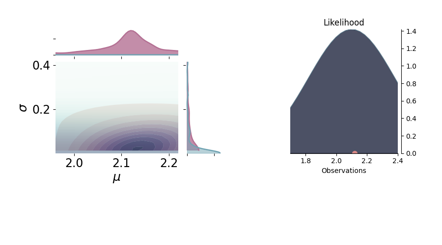
p = PlotPosterior(az_data)

p.create_figure(figsize=(9, 5), joyplot=False, marginal=True, likelihood=True)
p.plot_marginal(var_names=['$\mu$', '$\sigma$'],
                plot_trace=False, credible_interval=.93, kind='kde',
                joint_kwargs={'contour': True, 'pcolormesh_kwargs': {}},
                joint_kwargs_prior={'contour': False, 'pcolormesh_kwargs': {}})

p.axjoin.set_xlim(1.96, 2.22)
p.plot_normal_likelihood('$\mu$', '$\sigma$', '$y$', iteration=-6, hide_lines=True)
p.likelihood_axes.set_xlim(1.70, 2.40)
plt.show()

License

The code in this case study is copyrighted by Miguel de la Varga and licensed under the new BSD (3-clause) license:

https://opensource.org/licenses/BSD-3-Clause

The text and figures in this case study are copyrighted by Miguel de la Varga and licensed under the CC BY-NC 4.0 license:

https://creativecommons.org/licenses/by-nc/4.0/ Make sure to replace the links with actual hyperlinks if you’re using a platform that supports it (e.g., Markdown or HTML). Otherwise, the plain URLs work fine for plain text.