Simple example using Pyro: Moving the bell
We can sum up the workflow above in the following steps:
We chose a probabilistic density function family \(\pi\)—e.g., of the Gaussian or uniform families, \(\pi_S(\theta)\) to approximate the data generating process.
We narrow the possible values of \(\theta\)—mean and standard deviation in the case of a Normal distribution—with domain knowledge (notice that although \(\pi_S\) is a subset of \(\pi_P\), its size is infinite and therefore exhaustive approaches are unfeasible).
We use Bayesian inference to condition the prior estimations to our samples of reality \(\pi_S(\tilde{y})|\theta)\).
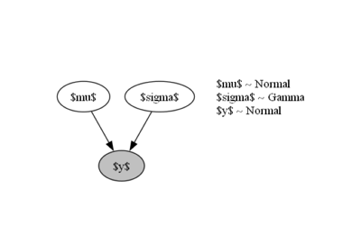
Back to the thickness example, we need to assign some prior distribution to the mean and standard deviation of the thickness; for example, we can take a naive approach and use the values of the crust, or on the contrary, we could use only the data we gathered and maybe one or two references. At this stage, there is not one single valid answer. To analyze how different priors affect, we will use 4 possible configurations, 2 of them using a normal distribution for the mean of a Gaussian likelihood function and the other 2 using a uniform distribution—between 0 and 10 in order to keep it as uninformative as possible while still giving valid physical values:
Normal |
Uniform |
|---|---|
\(\theta_\mu \sim \mathcal{N}(\mu=2.08, \sigma=0.07)\) |
\(\theta_\mu \sim \mathcal{U}(a=0, b=10)\) |
\(\theta_\sigma \sim \Gamma(\alpha=0.3, \beta=3)\) |
\(\theta_\sigma \sim \Gamma(=1.0, \beta=0.7)\) |
\(\pi_S(y|\theta) \sim \mathcal{N}(\mu=\theta_\mu, \sigma=\theta_\sigma)\) |
\(\pi_S(y|\theta) \sim \mathcal{N}(\mu=\theta_\mu, \sigma=\theta_\sigma)\) |
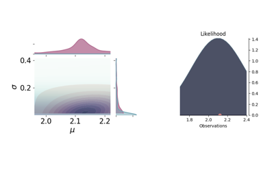
The standard deviation is in both cases a quite uninformative Gamma distribution. Besides using different probability functions to describe one of the model parameters, we have also repeated the same simulation either using one observation, \(\tilde{y}\) at 2.12 m, or 10 observation spread randomly (as random as a human possibly can) around 2.10. Figure fig-models1 shows the joint prior (in blue) and posterior (in red) distributions for the 4 probabilistic models, as well as, the maximum likelihood function.


