Normal Prior, single observation

# sphinx_gallery_thumbnail_number = -1

import arviz as az
import matplotlib.pyplot as plt
import pyro
import torch
from matplotlib.ticker import StrMethodFormatter

from gempy_probability.plot_posterior import PlotPosterior
from _aux_func import infer_model

y_obs = torch.tensor([2.12])
y_obs_list = torch.tensor([2.12, 2.06, 2.08, 2.05, 2.08, 2.09,
                           2.19, 2.07, 2.16, 2.11, 2.13, 1.92])
pyro.set_rng_seed(4003)

az_data = infer_model(
    distributions_family="normal_distribution",
    data=y_obs
)
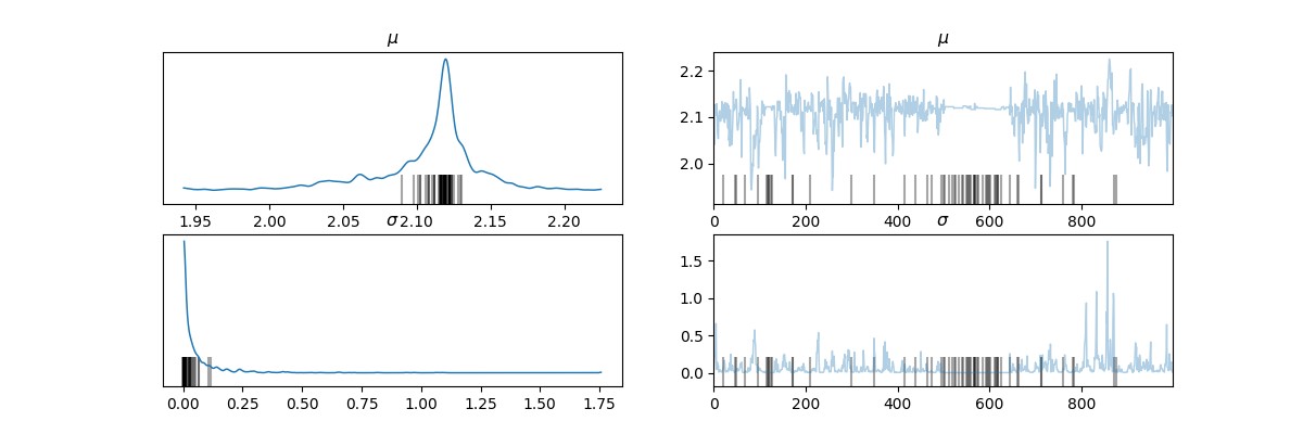
az.plot_trace(az_data)
plt.show()

Warmup:   0%|                                                       | 0/1100 [00:00, ?it/s]
Warmup:   2%|▎           | 25/1100 [00:00, 242.36it/s, step size=7.79e-02, acc. prob=0.761]
Warmup:   5%|▌           | 50/1100 [00:00, 155.16it/s, step size=5.05e-02, acc. prob=0.773]
Warmup:   6%|▋           | 68/1100 [00:00, 106.87it/s, step size=2.25e-02, acc. prob=0.772]
Warmup:   7%|▉            | 81/1100 [00:00, 82.62it/s, step size=2.71e-02, acc. prob=0.776]
Warmup:   9%|█▏           | 97/1100 [00:00, 97.36it/s, step size=1.45e-01, acc. prob=0.769]
Sample:  10%|█          | 112/1100 [00:01, 108.03it/s, step size=1.90e-01, acc. prob=0.982]
Sample:  12%|█▎         | 130/1100 [00:01, 124.11it/s, step size=1.90e-01, acc. prob=0.964]
Sample:  13%|█▍         | 148/1100 [00:01, 138.23it/s, step size=1.90e-01, acc. prob=0.945]
Sample:  15%|█▋         | 168/1100 [00:01, 153.82it/s, step size=1.90e-01, acc. prob=0.929]
Sample:  17%|█▉         | 190/1100 [00:01, 170.24it/s, step size=1.90e-01, acc. prob=0.932]
Sample:  19%|██▏        | 213/1100 [00:01, 184.87it/s, step size=1.90e-01, acc. prob=0.932]
Sample:  22%|██▍        | 240/1100 [00:01, 208.76it/s, step size=1.90e-01, acc. prob=0.832]
Sample:  24%|██▌        | 262/1100 [00:01, 194.96it/s, step size=1.90e-01, acc. prob=0.846]
Sample:  26%|██▊        | 283/1100 [00:01, 191.21it/s, step size=1.90e-01, acc. prob=0.852]
Sample:  28%|███        | 303/1100 [00:01, 186.75it/s, step size=1.90e-01, acc. prob=0.865]
Sample:  29%|███▏       | 323/1100 [00:02, 190.14it/s, step size=1.90e-01, acc. prob=0.868]
Sample:  31%|███▍       | 344/1100 [00:02, 193.28it/s, step size=1.90e-01, acc. prob=0.860]
Sample:  33%|███▋       | 364/1100 [00:02, 179.54it/s, step size=1.90e-01, acc. prob=0.869]
Sample:  35%|███▊       | 383/1100 [00:02, 178.39it/s, step size=1.90e-01, acc. prob=0.873]
Sample:  37%|████       | 402/1100 [00:02, 176.59it/s, step size=1.90e-01, acc. prob=0.879]
Sample:  38%|████▏      | 423/1100 [00:02, 182.61it/s, step size=1.90e-01, acc. prob=0.880]
Sample:  40%|████▍      | 442/1100 [00:02, 184.65it/s, step size=1.90e-01, acc. prob=0.885]
Sample:  42%|████▌      | 461/1100 [00:02, 181.63it/s, step size=1.90e-01, acc. prob=0.887]
Sample:  44%|████▊      | 480/1100 [00:02, 171.44it/s, step size=1.90e-01, acc. prob=0.887]
Sample:  45%|████▉      | 498/1100 [00:03, 172.83it/s, step size=1.90e-01, acc. prob=0.887]
Sample:  47%|█████▏     | 521/1100 [00:03, 186.95it/s, step size=1.90e-01, acc. prob=0.879]
Sample:  49%|█████▍     | 540/1100 [00:03, 182.67it/s, step size=1.90e-01, acc. prob=0.879]
Sample:  51%|█████▌     | 559/1100 [00:03, 183.52it/s, step size=1.90e-01, acc. prob=0.881]
Sample:  53%|█████▊     | 584/1100 [00:03, 201.97it/s, step size=1.90e-01, acc. prob=0.877]
Sample:  55%|██████     | 605/1100 [00:03, 202.68it/s, step size=1.90e-01, acc. prob=0.869]
Sample:  61%|██████▋    | 674/1100 [00:03, 343.16it/s, step size=1.90e-01, acc. prob=0.771]
Sample:  68%|███████▍   | 746/1100 [00:03, 452.91it/s, step size=1.90e-01, acc. prob=0.696]
Sample:  72%|███████▉   | 792/1100 [00:04, 298.81it/s, step size=1.90e-01, acc. prob=0.709]
Sample:  75%|████████▎  | 830/1100 [00:04, 236.29it/s, step size=1.90e-01, acc. prob=0.721]
Sample:  78%|████████▌  | 861/1100 [00:04, 221.68it/s, step size=1.90e-01, acc. prob=0.730]
Sample:  81%|████████▉  | 888/1100 [00:04, 216.90it/s, step size=1.90e-01, acc. prob=0.733]
Sample:  83%|█████████▏ | 913/1100 [00:04, 204.47it/s, step size=1.90e-01, acc. prob=0.740]
Sample:  85%|█████████▎ | 936/1100 [00:04, 200.75it/s, step size=1.90e-01, acc. prob=0.747]
Sample:  87%|█████████▌ | 958/1100 [00:05, 183.76it/s, step size=1.90e-01, acc. prob=0.753]
Sample:  89%|█████████▊ | 978/1100 [00:05, 181.71it/s, step size=1.90e-01, acc. prob=0.757]
Sample:  91%|█████████▉ | 999/1100 [00:05, 187.94it/s, step size=1.90e-01, acc. prob=0.758]
Sample:  93%|█████████▎| 1019/1100 [00:05, 182.27it/s, step size=1.90e-01, acc. prob=0.762]
Sample:  94%|█████████▍| 1038/1100 [00:05, 176.88it/s, step size=1.90e-01, acc. prob=0.766]
Sample:  96%|█████████▌| 1056/1100 [00:05, 173.28it/s, step size=1.90e-01, acc. prob=0.769]
Sample:  98%|█████████▊| 1075/1100 [00:05, 174.55it/s, step size=1.90e-01, acc. prob=0.773]
Sample:  99%|█████████▉| 1093/1100 [00:05, 169.94it/s, step size=1.90e-01, acc. prob=0.777]
Sample: 100%|██████████| 1100/1100 [00:05, 187.01it/s, step size=1.90e-01, acc. prob=0.778]

posterior predictive shape not compatible with number of chains and draws.This can mean that some draws or even whole chains are not represented.

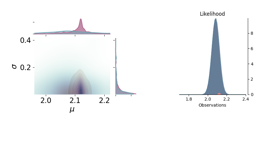
p = PlotPosterior(az_data)

p.create_figure(figsize=(9, 5), joyplot=False, marginal=True, likelihood=True)
p.plot_marginal(var_names=['$\mu$', '$\sigma$'],
                plot_trace=False, credible_interval=.93, kind='kde',
                joint_kwargs={'contour': True, 'pcolormesh_kwargs': {}},
                joint_kwargs_prior={'contour': False, 'pcolormesh_kwargs': {}})

p.axjoin.set_xlim(1.96, 2.22)
p.plot_normal_likelihood('$\mu$', '$\sigma$', '$y$', iteration=-6, hide_lines=True)
p.likelihood_axes.set_xlim(1.70, 2.40)
plt.show()

License

The code in this case study is copyrighted by Miguel de la Varga and licensed under the new BSD (3-clause) license:

https://opensource.org/licenses/BSD-3-Clause

The text and figures in this case study are copyrighted by Miguel de la Varga and licensed under the CC BY-NC 4.0 license:

https://creativecommons.org/licenses/by-nc/4.0/ Make sure to replace the links with actual hyperlinks if you’re using a platform that supports it (e.g., Markdown or HTML). Otherwise, the plain URLs work fine for plain text.