Note

Go to the end to download the full example code

2.1 - Only Pyro¶

Model definition¶

Same problem as before, let’s assume the observations are layer thickness measurements taken on an outcrop. Now, in the previous example we chose a prior for the mean arbitrarily: $𝜇∼Normal(mu=10.0, sigma=5.0)$–something that made sense for these specific data set. If we do not have any further information, keeping an uninformative prior and let the data to dictate the final value of the inference is the sensible way forward. However, this also enable to add information to the system by setting informative priors.

Imagine we get a borehole with the tops of the two interfaces of interest. Each of this data point will be a random variable itself since the accuracy of the exact 3D location will be always limited. Notice that this two data points refer to depth not to thickness–the unit of the rest of the observations. Therefore, the first step would be to perform a transformation of the parameters into the observations space. Naturally in this example a simple subtraction will suffice.

Now we can define the probabilistic models:

# sphinx_gallery_thumbnail_number = -2

Importing Necessary Libraries¶

import os
import io
from PIL import Image
import matplotlib.pyplot as plt
import pyro
import pyro.distributions as dist
import torch
from pyro.infer import MCMC, NUTS, Predictive
from pyro.infer.inspect import get_dependencies
from gempy_probability.plot_posterior import PlotPosterior, default_red, default_blue
import arviz as az

az.style.use("arviz-doc")

Introduction to the Problem¶

In this example, we are considering layer thickness measurements taken on an outcrop as our observations. We use a probabilistic approach to model these observations, allowing for the inclusion of prior knowledge and uncertainty quantification.

# Setting the working directory for sphinx gallery
cwd = os.getcwd()
if 'examples' not in cwd:
    path_dir = os.getcwd() + '/examples/tutorials/ch5_probabilistic_modeling'
else:
    path_dir = cwd

Defining the Observations and Model¶

The observations are layer thickness measurements. We define a Pyro probabilistic model that uses Normal and Gamma distributions to model the top and bottom interfaces of the layers and their respective uncertainties.

# Defining observed data
y_obs = torch.tensor([2.12])
y_obs_list = torch.tensor([2.12, 2.06, 2.08, 2.05, 2.08, 2.09, 2.19, 2.07, 2.16, 2.11, 2.13, 1.92])
pyro.set_rng_seed(4003)


# Defining the probabilistic model
def model(y_obs_list_):
    mu_top = pyro.sample(r'$\mu_{top}$', dist.Normal(3.05, 0.2))
    sigma_top = pyro.sample(r"$\sigma_{top}$", dist.Gamma(0.3, 3.0))
    y_top = pyro.sample(r"y_{top}", dist.Normal(mu_top, sigma_top), obs=torch.tensor([3.02]))

    mu_bottom = pyro.sample(r'$\mu_{bottom}$', dist.Normal(1.02, 0.2))
    sigma_bottom = pyro.sample(r'$\sigma_{bottom}$', dist.Gamma(0.3, 3.0))
    y_bottom = pyro.sample(r'y_{bottom}', dist.Normal(mu_bottom, sigma_bottom), obs=torch.tensor([1.02]))

    mu_thickness = pyro.deterministic(r'$\mu_{thickness}$', mu_top - mu_bottom)
    sigma_thickness = pyro.sample(r'$\sigma_{thickness}$', dist.Gamma(0.3, 3.0))
    y_thickness = pyro.sample(r'y_{thickness}', dist.Normal(mu_thickness, sigma_thickness), obs=y_obs_list_)


# Exploring model dependencies
dependencies = get_dependencies(model, model_args=y_obs_list[:1])
dependencies

{'prior_dependencies': {'$\\mu_{top}$': {'$\\mu_{top}$': set()}, '$\\sigma_{top}$': {'$\\sigma_{top}$': set()}, 'y_{top}': {'y_{top}': set(), '$\\mu_{top}$': set(), '$\\sigma_{top}$': set()}, '$\\mu_{bottom}$': {'$\\mu_{bottom}$': set()}, '$\\sigma_{bottom}$': {'$\\sigma_{bottom}$': set()}, 'y_{bottom}': {'y_{bottom}': set(), '$\\mu_{bottom}$': set(), '$\\sigma_{bottom}$': set()}, '$\\sigma_{thickness}$': {'$\\sigma_{thickness}$': set()}, 'y_{thickness}': {'y_{thickness}': set(), '$\\mu_{top}$': set(), '$\\mu_{bottom}$': set(), '$\\sigma_{thickness}$': set()}}, 'posterior_dependencies': {'$\\mu_{top}$': {'$\\mu_{top}$': set(), 'y_{top}': set(), 'y_{thickness}': set(), '$\\sigma_{top}$': set(), '$\\mu_{bottom}$': set(), '$\\sigma_{thickness}$': set()}, '$\\sigma_{top}$': {'$\\sigma_{top}$': set(), 'y_{top}': set()}, '$\\mu_{bottom}$': {'$\\mu_{bottom}$': set(), 'y_{bottom}': set(), 'y_{thickness}': set(), '$\\sigma_{bottom}$': set(), '$\\sigma_{thickness}$': set()}, '$\\sigma_{bottom}$': {'$\\sigma_{bottom}$': set(), 'y_{bottom}': set()}, '$\\sigma_{thickness}$': {'$\\sigma_{thickness}$': set(), 'y_{thickness}': set()}}}

graph = pyro.render_model(
    model=model,
    model_args=(y_obs_list,),
    render_params=True,
    render_distributions=True,
    render_deterministic=True
)

graph.attr(dpi='300')
# Convert the graph to a PNG image format
s = graph.pipe(format='png')

# Open the image with PIL
image = Image.open(io.BytesIO(s))

# Plot the image with matplotlib
plt.figure(figsize=(10, 4))
plt.imshow(image)
plt.axis('off')  # Turn off axis
plt.show()

Prior Sampling¶

Prior sampling is performed to understand the initial distribution of the model parameters before considering the observed data.

# Prior sampling
num_samples= 500
prior = Predictive(model, num_samples=num_samples)(y_obs_list)

Running MCMC Sampling¶

Markov Chain Monte Carlo (MCMC) sampling is used to sample from the posterior distribution, providing insights into the distribution of model parameters after considering the observed data.

# Running MCMC using the NUTS algorithm
nuts_kernel = NUTS(model)
mcmc = MCMC(nuts_kernel, num_samples=num_samples, warmup_steps=100)
mcmc.run(y_obs_list)

Warmup:   0%|          | 0/600 [00:00, ?it/s]
Warmup:   1%|▏         | 8/600 [00:00, 56.83it/s, step size=2.95e-02, acc. prob=0.651]
Warmup:   2%|▏         | 14/600 [00:00, 12.46it/s, step size=5.85e-03, acc. prob=0.677]
Warmup:   3%|▎         | 17/600 [00:01, 11.19it/s, step size=1.03e-02, acc. prob=0.708]
Warmup:   3%|▎         | 19/600 [00:01,  9.20it/s, step size=1.69e-02, acc. prob=0.725]
Warmup:   4%|▎         | 21/600 [00:01,  9.91it/s, step size=2.54e-02, acc. prob=0.737]
Warmup:   4%|▍         | 23/600 [00:02,  6.16it/s, step size=4.74e-03, acc. prob=0.717]
Warmup:   4%|▍         | 24/600 [00:02,  5.02it/s, step size=8.42e-03, acc. prob=0.728]
Warmup:   4%|▍         | 25/600 [00:03,  5.12it/s, step size=1.10e-02, acc. prob=0.734]
Warmup:   4%|▍         | 26/600 [00:03,  4.44it/s, step size=1.22e-02, acc. prob=0.737]
Warmup:   5%|▍         | 29/600 [00:03,  6.45it/s, step size=2.21e-02, acc. prob=0.750]
Warmup:   6%|▌         | 33/600 [00:04,  6.36it/s, step size=1.09e-02, acc. prob=0.746]
Warmup:   6%|▌         | 37/600 [00:04,  8.74it/s, step size=8.45e-03, acc. prob=0.748]
Warmup:   6%|▋         | 39/600 [00:05,  5.46it/s, step size=1.45e-02, acc. prob=0.755]
Warmup:   7%|▋         | 43/600 [00:05,  7.24it/s, step size=6.67e-03, acc. prob=0.751]
Warmup:   8%|▊         | 45/600 [00:05,  7.08it/s, step size=1.03e-02, acc. prob=0.756]
Warmup:   8%|▊         | 49/600 [00:06,  7.18it/s, step size=9.30e-03, acc. prob=0.758]
Warmup:   8%|▊         | 50/600 [00:06,  5.95it/s, step size=1.54e-02, acc. prob=0.763]
Warmup:   8%|▊         | 51/600 [00:06,  6.28it/s, step size=2.49e-02, acc. prob=0.767]
Warmup:   9%|▉         | 54/600 [00:07,  8.93it/s, step size=8.63e-03, acc. prob=0.760]
Warmup:   9%|▉         | 56/600 [00:07,  9.50it/s, step size=1.40e-02, acc. prob=0.765]
Warmup:  10%|█         | 60/600 [00:07, 14.10it/s, step size=7.29e-03, acc. prob=0.761]
Warmup:  10%|█         | 63/600 [00:07, 13.13it/s, step size=2.61e-02, acc. prob=0.772]
Warmup:  11%|█         | 65/600 [00:07, 12.17it/s, step size=1.84e-02, acc. prob=0.770]
Warmup:  11%|█         | 67/600 [00:08, 11.15it/s, step size=2.33e-02, acc. prob=0.772]
Warmup:  12%|█▏        | 71/600 [00:08, 13.88it/s, step size=9.51e-03, acc. prob=0.767]
Warmup:  12%|█▏        | 73/600 [00:08, 10.43it/s, step size=1.23e-02, acc. prob=0.769]
Warmup:  13%|█▎        | 77/600 [00:08, 14.18it/s, step size=8.53e-03, acc. prob=0.768]
Warmup:  13%|█▎        | 79/600 [00:08, 11.89it/s, step size=1.14e-02, acc. prob=0.770]
Warmup:  14%|█▎        | 81/600 [00:09,  9.17it/s, step size=7.80e-03, acc. prob=0.768]
Warmup:  14%|█▍        | 83/600 [00:09,  7.62it/s, step size=1.67e-02, acc. prob=0.773]
Warmup:  14%|█▍        | 86/600 [00:10,  6.38it/s, step size=9.87e-03, acc. prob=0.771]
Warmup:  15%|█▍        | 88/600 [00:10,  7.41it/s, step size=6.44e-03, acc. prob=0.769]
Warmup:  15%|█▌        | 90/600 [00:11,  4.18it/s, step size=7.07e-01, acc. prob=0.763]
Warmup:  16%|█▌        | 93/600 [00:11,  6.07it/s, step size=9.36e-02, acc. prob=0.759]
Warmup:  16%|█▋        | 98/600 [00:11, 10.09it/s, step size=2.54e-02, acc. prob=0.758]
Warmup:  17%|█▋        | 101/600 [00:12, 10.79it/s, step size=7.32e-02, acc. prob=0.942]
Sample:  18%|█▊        | 105/600 [00:12, 14.41it/s, step size=7.32e-02, acc. prob=0.981]
Sample:  18%|█▊        | 111/600 [00:12, 19.89it/s, step size=7.32e-02, acc. prob=0.971]
Sample:  19%|█▉        | 114/600 [00:12, 21.07it/s, step size=7.32e-02, acc. prob=0.975]
Sample:  20%|█▉        | 118/600 [00:12, 23.87it/s, step size=7.32e-02, acc. prob=0.968]
Sample:  20%|██        | 122/600 [00:12, 21.94it/s, step size=7.32e-02, acc. prob=0.969]
Sample:  21%|██        | 125/600 [00:12, 22.11it/s, step size=7.32e-02, acc. prob=0.958]
Sample:  21%|██▏       | 128/600 [00:12, 22.68it/s, step size=7.32e-02, acc. prob=0.962]
Sample:  22%|██▏       | 131/600 [00:13, 23.65it/s, step size=7.32e-02, acc. prob=0.962]
Sample:  22%|██▏       | 134/600 [00:13, 21.79it/s, step size=7.32e-02, acc. prob=0.964]
Sample:  23%|██▎       | 138/600 [00:13, 22.56it/s, step size=7.32e-02, acc. prob=0.967]
Sample:  24%|██▎       | 141/600 [00:13, 22.47it/s, step size=7.32e-02, acc. prob=0.969]
Sample:  24%|██▍       | 145/600 [00:13, 25.63it/s, step size=7.32e-02, acc. prob=0.969]
Sample:  25%|██▍       | 148/600 [00:13, 23.61it/s, step size=7.32e-02, acc. prob=0.970]
Sample:  25%|██▌       | 151/600 [00:13, 21.54it/s, step size=7.32e-02, acc. prob=0.969]
Sample:  26%|██▌       | 155/600 [00:14, 23.93it/s, step size=7.32e-02, acc. prob=0.969]
Sample:  27%|██▋       | 160/600 [00:14, 29.28it/s, step size=7.32e-02, acc. prob=0.941]
Sample:  27%|██▋       | 164/600 [00:14, 27.67it/s, step size=7.32e-02, acc. prob=0.944]
Sample:  28%|██▊       | 167/600 [00:14, 27.60it/s, step size=7.32e-02, acc. prob=0.944]
Sample:  28%|██▊       | 170/600 [00:14, 24.02it/s, step size=7.32e-02, acc. prob=0.944]
Sample:  29%|██▉       | 173/600 [00:14, 23.55it/s, step size=7.32e-02, acc. prob=0.934]
Sample:  30%|██▉       | 177/600 [00:14, 26.45it/s, step size=7.32e-02, acc. prob=0.929]
Sample:  30%|███       | 180/600 [00:15, 24.85it/s, step size=7.32e-02, acc. prob=0.925]
Sample:  30%|███       | 183/600 [00:15, 23.97it/s, step size=7.32e-02, acc. prob=0.928]
Sample:  31%|███       | 186/600 [00:15, 24.93it/s, step size=7.32e-02, acc. prob=0.929]
Sample:  32%|███▏      | 189/600 [00:15, 23.35it/s, step size=7.32e-02, acc. prob=0.929]
Sample:  32%|███▏      | 192/600 [00:15, 22.07it/s, step size=7.32e-02, acc. prob=0.932]
Sample:  32%|███▎      | 195/600 [00:15, 19.26it/s, step size=7.32e-02, acc. prob=0.932]
Sample:  33%|███▎      | 198/600 [00:15, 20.71it/s, step size=7.32e-02, acc. prob=0.930]
Sample:  34%|███▍      | 203/600 [00:16, 26.94it/s, step size=7.32e-02, acc. prob=0.931]
Sample:  34%|███▍      | 207/600 [00:16, 28.33it/s, step size=7.32e-02, acc. prob=0.933]
Sample:  35%|███▌      | 211/600 [00:16, 26.17it/s, step size=7.32e-02, acc. prob=0.935]
Sample:  36%|███▌      | 214/600 [00:16, 26.08it/s, step size=7.32e-02, acc. prob=0.935]
Sample:  37%|███▋      | 220/600 [00:16, 33.50it/s, step size=7.32e-02, acc. prob=0.920]
Sample:  37%|███▋      | 224/600 [00:16, 29.03it/s, step size=7.32e-02, acc. prob=0.919]
Sample:  38%|███▊      | 228/600 [00:16, 29.87it/s, step size=7.32e-02, acc. prob=0.921]
Sample:  39%|███▉      | 233/600 [00:16, 34.03it/s, step size=7.32e-02, acc. prob=0.921]
Sample:  40%|███▉      | 237/600 [00:17, 34.15it/s, step size=7.32e-02, acc. prob=0.921]
Sample:  40%|████      | 241/600 [00:17, 33.51it/s, step size=7.32e-02, acc. prob=0.920]
Sample:  41%|████      | 245/600 [00:17, 28.09it/s, step size=7.32e-02, acc. prob=0.922]
Sample:  42%|████▏     | 250/600 [00:17, 32.69it/s, step size=7.32e-02, acc. prob=0.923]
Sample:  42%|████▏     | 254/600 [00:17, 27.87it/s, step size=7.32e-02, acc. prob=0.918]
Sample:  43%|████▎     | 258/600 [00:17, 26.77it/s, step size=7.32e-02, acc. prob=0.912]
Sample:  44%|████▎     | 261/600 [00:18, 26.32it/s, step size=7.32e-02, acc. prob=0.906]
Sample:  44%|████▍     | 264/600 [00:18, 25.25it/s, step size=7.32e-02, acc. prob=0.907]
Sample:  44%|████▍     | 267/600 [00:18, 26.17it/s, step size=7.32e-02, acc. prob=0.908]
Sample:  45%|████▌     | 270/600 [00:18, 25.31it/s, step size=7.32e-02, acc. prob=0.910]
Sample:  46%|████▌     | 273/600 [00:18, 25.42it/s, step size=7.32e-02, acc. prob=0.911]
Sample:  46%|████▌     | 276/600 [00:18, 19.99it/s, step size=7.32e-02, acc. prob=0.911]
Sample:  47%|████▋     | 280/600 [00:18, 22.44it/s, step size=7.32e-02, acc. prob=0.913]
Sample:  47%|████▋     | 284/600 [00:18, 24.84it/s, step size=7.32e-02, acc. prob=0.913]
Sample:  48%|████▊     | 288/600 [00:19, 26.21it/s, step size=7.32e-02, acc. prob=0.915]
Sample:  49%|████▊     | 292/600 [00:19, 29.01it/s, step size=7.32e-02, acc. prob=0.916]
Sample:  49%|████▉     | 296/600 [00:19, 29.02it/s, step size=7.32e-02, acc. prob=0.914]
Sample:  50%|█████     | 303/600 [00:19, 36.99it/s, step size=7.32e-02, acc. prob=0.895]
Sample:  51%|█████     | 307/600 [00:19, 31.63it/s, step size=7.32e-02, acc. prob=0.895]
Sample:  52%|█████▏    | 311/600 [00:19, 25.95it/s, step size=7.32e-02, acc. prob=0.896]
Sample:  53%|█████▎    | 316/600 [00:20, 28.37it/s, step size=7.32e-02, acc. prob=0.894]
Sample:  53%|█████▎    | 320/600 [00:20, 29.10it/s, step size=7.32e-02, acc. prob=0.896]
Sample:  54%|█████▍    | 324/600 [00:20, 31.02it/s, step size=7.32e-02, acc. prob=0.896]
Sample:  55%|█████▍    | 328/600 [00:20, 30.18it/s, step size=7.32e-02, acc. prob=0.897]
Sample:  55%|█████▌    | 332/600 [00:20, 27.72it/s, step size=7.32e-02, acc. prob=0.896]
Sample:  56%|█████▌    | 335/600 [00:20, 26.97it/s, step size=7.32e-02, acc. prob=0.897]
Sample:  56%|█████▋    | 339/600 [00:20, 29.62it/s, step size=7.32e-02, acc. prob=0.897]
Sample:  57%|█████▋    | 343/600 [00:21, 22.69it/s, step size=7.32e-02, acc. prob=0.899]
Sample:  58%|█████▊    | 346/600 [00:21, 22.78it/s, step size=7.32e-02, acc. prob=0.899]
Sample:  58%|█████▊    | 349/600 [00:21, 23.84it/s, step size=7.32e-02, acc. prob=0.900]
Sample:  59%|█████▊    | 352/600 [00:21, 22.75it/s, step size=7.32e-02, acc. prob=0.901]
Sample:  59%|█████▉    | 356/600 [00:21, 25.78it/s, step size=7.32e-02, acc. prob=0.895]
Sample:  60%|██████    | 360/600 [00:21, 25.55it/s, step size=7.32e-02, acc. prob=0.891]
Sample:  60%|██████    | 363/600 [00:21, 23.50it/s, step size=7.32e-02, acc. prob=0.892]
Sample:  61%|██████    | 366/600 [00:22, 24.35it/s, step size=7.32e-02, acc. prob=0.893]
Sample:  62%|██████▏   | 370/600 [00:22, 27.28it/s, step size=7.32e-02, acc. prob=0.894]
Sample:  62%|██████▏   | 373/600 [00:22, 27.07it/s, step size=7.32e-02, acc. prob=0.895]
Sample:  63%|██████▎   | 380/600 [00:22, 37.62it/s, step size=7.32e-02, acc. prob=0.883]
Sample:  64%|██████▍   | 384/600 [00:22, 30.04it/s, step size=7.32e-02, acc. prob=0.884]
Sample:  65%|██████▍   | 388/600 [00:22, 30.84it/s, step size=7.32e-02, acc. prob=0.884]
Sample:  65%|██████▌   | 392/600 [00:22, 28.30it/s, step size=7.32e-02, acc. prob=0.886]
Sample:  66%|██████▌   | 396/600 [00:22, 29.84it/s, step size=7.32e-02, acc. prob=0.887]
Sample:  67%|██████▋   | 400/600 [00:23, 30.31it/s, step size=7.32e-02, acc. prob=0.888]
Sample:  67%|██████▋   | 404/600 [00:23, 32.24it/s, step size=7.32e-02, acc. prob=0.889]
Sample:  68%|██████▊   | 408/600 [00:23, 30.19it/s, step size=7.32e-02, acc. prob=0.886]
Sample:  69%|██████▊   | 412/600 [00:23, 30.89it/s, step size=7.32e-02, acc. prob=0.887]
Sample:  69%|██████▉   | 416/600 [00:23, 32.16it/s, step size=7.32e-02, acc. prob=0.888]
Sample:  70%|███████   | 420/600 [00:23, 28.63it/s, step size=7.32e-02, acc. prob=0.889]
Sample:  71%|███████   | 424/600 [00:23, 27.88it/s, step size=7.32e-02, acc. prob=0.889]
Sample:  71%|███████▏  | 428/600 [00:24, 29.00it/s, step size=7.32e-02, acc. prob=0.890]
Sample:  72%|███████▏  | 431/600 [00:24, 29.03it/s, step size=7.32e-02, acc. prob=0.891]
Sample:  73%|███████▎  | 436/600 [00:24, 30.35it/s, step size=7.32e-02, acc. prob=0.891]
Sample:  73%|███████▎  | 440/600 [00:24, 26.99it/s, step size=7.32e-02, acc. prob=0.892]
Sample:  74%|███████▍  | 444/600 [00:24, 28.00it/s, step size=7.32e-02, acc. prob=0.893]
Sample:  74%|███████▍  | 447/600 [00:24, 24.89it/s, step size=7.32e-02, acc. prob=0.894]
Sample:  75%|███████▌  | 451/600 [00:24, 24.46it/s, step size=7.32e-02, acc. prob=0.894]
Sample:  76%|███████▌  | 455/600 [00:25, 23.06it/s, step size=7.32e-02, acc. prob=0.895]
Sample:  76%|███████▋  | 458/600 [00:25, 23.81it/s, step size=7.32e-02, acc. prob=0.896]
Sample:  77%|███████▋  | 461/600 [00:25, 21.70it/s, step size=7.32e-02, acc. prob=0.896]
Sample:  77%|███████▋  | 464/600 [00:25, 18.56it/s, step size=7.32e-02, acc. prob=0.896]
Sample:  78%|███████▊  | 466/600 [00:25, 18.69it/s, step size=7.32e-02, acc. prob=0.896]
Sample:  78%|███████▊  | 470/600 [00:25, 22.64it/s, step size=7.32e-02, acc. prob=0.896]
Sample:  79%|███████▉  | 474/600 [00:25, 24.91it/s, step size=7.32e-02, acc. prob=0.897]
Sample:  80%|███████▉  | 477/600 [00:26, 25.65it/s, step size=7.32e-02, acc. prob=0.897]
Sample:  80%|████████  | 480/600 [00:26, 25.38it/s, step size=7.32e-02, acc. prob=0.898]
Sample:  81%|████████  | 484/600 [00:26, 26.93it/s, step size=7.32e-02, acc. prob=0.899]
Sample:  81%|████████  | 487/600 [00:26, 25.53it/s, step size=7.32e-02, acc. prob=0.898]
Sample:  82%|████████▏ | 490/600 [00:26, 26.59it/s, step size=7.32e-02, acc. prob=0.898]
Sample:  82%|████████▏ | 493/600 [00:26, 22.86it/s, step size=7.32e-02, acc. prob=0.899]
Sample:  83%|████████▎ | 496/600 [00:26, 23.02it/s, step size=7.32e-02, acc. prob=0.899]
Sample:  83%|████████▎ | 499/600 [00:27, 22.87it/s, step size=7.32e-02, acc. prob=0.900]
Sample:  84%|████████▍ | 504/600 [00:27, 27.58it/s, step size=7.32e-02, acc. prob=0.897]
Sample:  85%|████████▍ | 508/600 [00:27, 29.17it/s, step size=7.32e-02, acc. prob=0.898]
Sample:  85%|████████▌ | 511/600 [00:27, 26.39it/s, step size=7.32e-02, acc. prob=0.898]
Sample:  86%|████████▌ | 514/600 [00:27, 25.46it/s, step size=7.32e-02, acc. prob=0.899]
Sample:  86%|████████▋ | 518/600 [00:27, 26.15it/s, step size=7.32e-02, acc. prob=0.900]
Sample:  87%|████████▋ | 521/600 [00:27, 25.74it/s, step size=7.32e-02, acc. prob=0.898]
Sample:  88%|████████▊ | 525/600 [00:27, 26.85it/s, step size=7.32e-02, acc. prob=0.899]
Sample:  88%|████████▊ | 529/600 [00:28, 29.09it/s, step size=7.32e-02, acc. prob=0.900]
Sample:  89%|████████▊ | 532/600 [00:28, 25.84it/s, step size=7.32e-02, acc. prob=0.900]
Sample:  89%|████████▉ | 535/600 [00:28, 24.08it/s, step size=7.32e-02, acc. prob=0.900]
Sample:  90%|████████▉ | 538/600 [00:28, 20.75it/s, step size=7.32e-02, acc. prob=0.901]
Sample:  90%|█████████ | 542/600 [00:28, 23.66it/s, step size=7.32e-02, acc. prob=0.902]
Sample:  91%|█████████ | 545/600 [00:28, 21.88it/s, step size=7.32e-02, acc. prob=0.902]
Sample:  92%|█████████▏| 549/600 [00:29, 22.89it/s, step size=7.32e-02, acc. prob=0.903]
Sample:  92%|█████████▏| 553/600 [00:29, 23.54it/s, step size=7.32e-02, acc. prob=0.904]
Sample:  93%|█████████▎| 556/600 [00:29, 23.46it/s, step size=7.32e-02, acc. prob=0.903]
Sample:  93%|█████████▎| 559/600 [00:29, 24.52it/s, step size=7.32e-02, acc. prob=0.903]
Sample:  94%|█████████▎| 562/600 [00:29, 23.30it/s, step size=7.32e-02, acc. prob=0.904]
Sample:  94%|█████████▍| 565/600 [00:29, 24.65it/s, step size=7.32e-02, acc. prob=0.904]
Sample:  95%|█████████▍| 569/600 [00:29, 27.72it/s, step size=7.32e-02, acc. prob=0.905]
Sample:  95%|█████████▌| 572/600 [00:29, 22.90it/s, step size=7.32e-02, acc. prob=0.906]
Sample:  96%|█████████▌| 575/600 [00:30, 22.74it/s, step size=7.32e-02, acc. prob=0.906]
Sample:  96%|█████████▋| 579/600 [00:30, 26.09it/s, step size=7.32e-02, acc. prob=0.906]
Sample:  97%|█████████▋| 582/600 [00:30, 24.75it/s, step size=7.32e-02, acc. prob=0.907]
Sample:  98%|█████████▊| 585/600 [00:30, 23.61it/s, step size=7.32e-02, acc. prob=0.907]
Sample:  98%|█████████▊| 588/600 [00:30, 23.21it/s, step size=7.32e-02, acc. prob=0.907]
Sample:  98%|█████████▊| 591/600 [00:30, 24.09it/s, step size=7.32e-02, acc. prob=0.907]
Sample:  99%|█████████▉| 595/600 [00:30, 25.30it/s, step size=7.32e-02, acc. prob=0.907]
Sample: 100%|█████████▉| 599/600 [00:30, 28.41it/s, step size=7.32e-02, acc. prob=0.907]
Sample: 100%|██████████| 600/600 [00:30, 19.36it/s, step size=7.32e-02, acc. prob=0.908]

Posterior Predictive Sampling¶

After obtaining the posterior samples, we perform posterior predictive sampling. This step allows us to make predictions based on the posterior distribution.

# Sampling from the posterior predictive distribution
posterior_samples = mcmc.get_samples(num_samples)
posterior_predictive = Predictive(model, posterior_samples)(y_obs_list)

Visualizing the Results¶

We use ArviZ, a library for exploratory analysis of Bayesian models, to visualize the results of our probabilistic model.

# Creating a data object for ArviZ
data = az.from_pyro(
    posterior=mcmc,
    prior=prior,
    posterior_predictive=posterior_predictive
)

# Plotting trace of the sampled parameters
az.plot_trace(data, kind="trace", figsize=(10, 10), compact=False)
plt.show()

$\mu_{bottom}$, $\mu_{bottom}$, $\mu_{top}$, $\mu_{top}$, $\sigma_{bottom}$, $\sigma_{bottom}$, $\sigma_{thickness}$, $\sigma_{thickness}$, $\sigma_{top}$, $\sigma_{top}$

/home/leguark/.virtualenvs/gempy_dependencies/lib/python3.10/site-packages/arviz/data/io_pyro.py:158: UserWarning: Could not get vectorized trace, log_likelihood group will be omitted. Check your model vectorization or set log_likelihood=False
  warnings.warn(

Plotting trace of the sampled parameters

az.plot_trace(posterior_predictive, var_names= (r"$\mu_{thickness}$"), kind="trace")
plt.show()

$\mu_{thickness}$, $\mu_{thickness}$

/home/leguark/.virtualenvs/gempy_dependencies/lib/python3.10/site-packages/arviz/data/base.py:265: UserWarning: More chains (500) than draws (1). Passed array should have shape (chains, draws, *shape)
  warnings.warn(
/home/leguark/.virtualenvs/gempy_dependencies/lib/python3.10/site-packages/arviz/data/base.py:265: UserWarning: More chains (500) than draws (12). Passed array should have shape (chains, draws, *shape)
  warnings.warn(
/home/leguark/.virtualenvs/gempy_dependencies/lib/python3.10/site-packages/arviz/stats/density_utils.py:488: UserWarning: Your data appears to have a single value or no finite values
  warnings.warn("Your data appears to have a single value or no finite values")

Density Plots of Posterior and Prior¶

Density plots provide a visual representation of the distribution of the sampled parameters. Comparing the posterior and prior distributions allows us to assess the impact of the observed data.

# Plotting density of posterior and prior distributions
az.plot_density(
    data=[data, data.prior],
    hdi_prob=0.95,
    shade=.2,
    data_labels=["Posterior", "Prior"],
    colors=[default_red, default_blue],
)


plt.show()

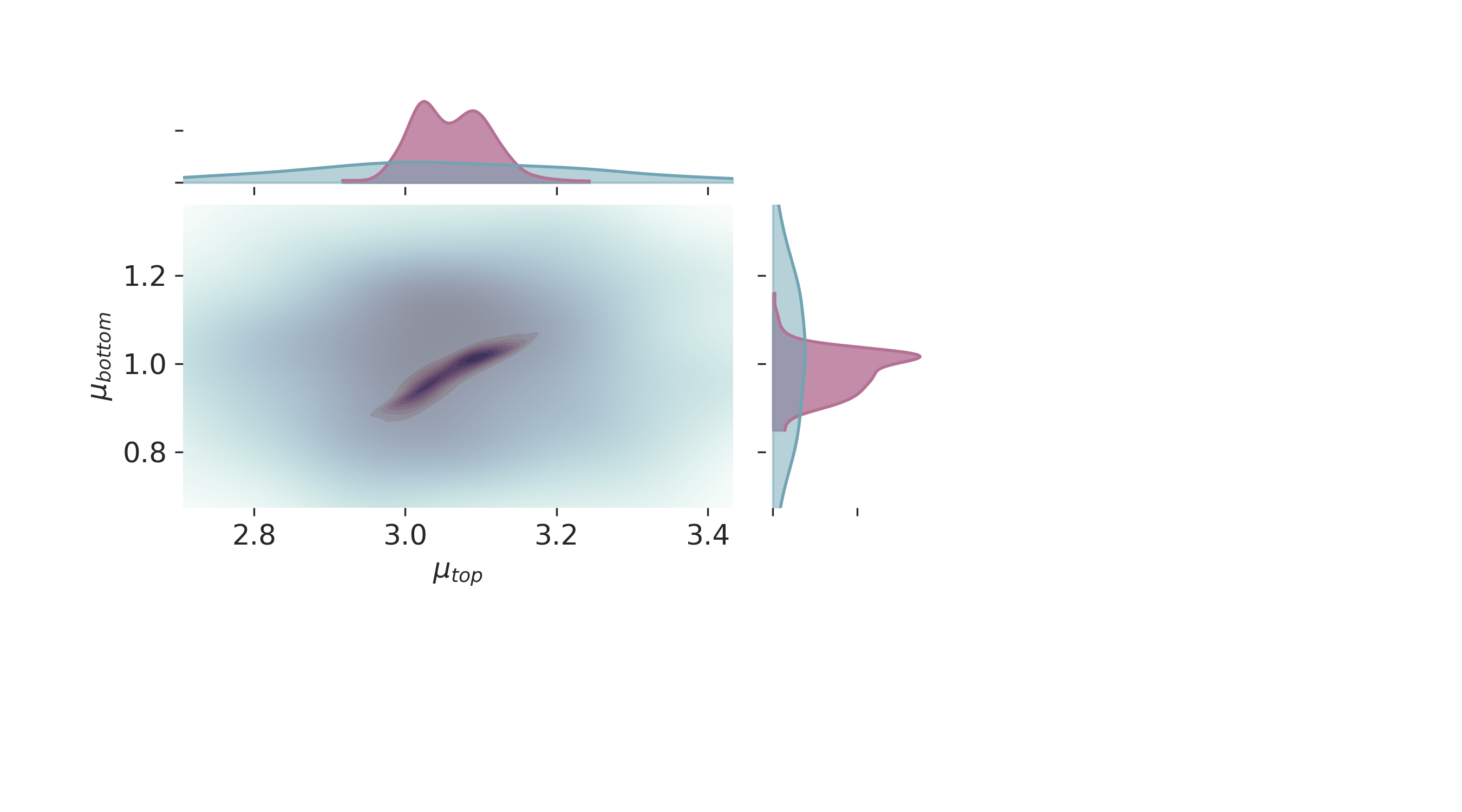
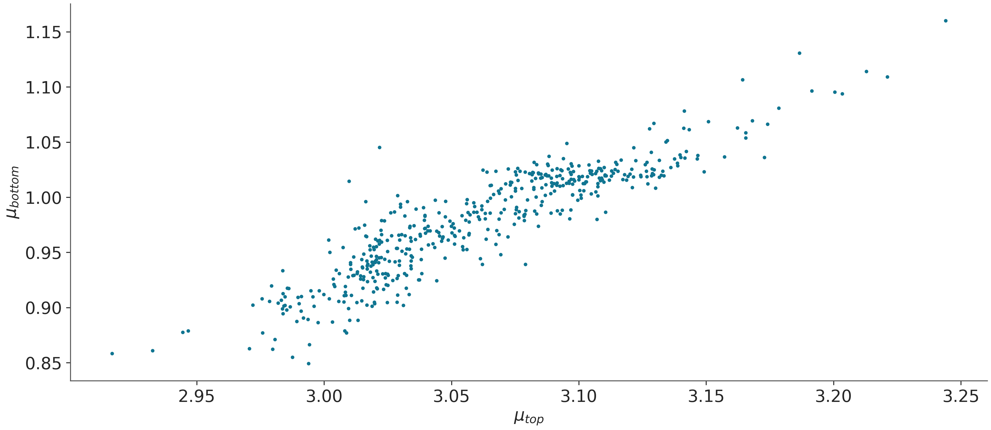
$\mu_{bottom}$, $\mu_{top}$, $\sigma_{bottom}$, $\sigma_{thickness}$, $\sigma_{top}$

Can we see a correlation between the posteriors of $mu_{bottom}$ and $mu_{top}$?

Density Plots of Posterior Predictive and Prior Predictive¶

These plots show the distribution of the posterior predictive and prior predictive checks. They help in evaluating the performance and validity of the probabilistic model.

# Plotting density of posterior predictive and prior predictive
az.plot_density(
    data=[data.posterior_predictive, data.prior_predictive],
    shade=.2,
    var_names=[r'$\mu_{thickness}$'],
    data_labels=["Posterior Predictive", "Prior Predictive"],
    colors=[default_red, default_blue],
    hdi_prob=0.90
)
plt.show()

$\mu_{thickness}$

Marginal Distribution Plots¶

Marginal distribution plots provide insights into the distribution of individual parameters. These plots help in understanding the uncertainty and variability in the parameter estimates.

# Creating marginal distribution plots
p = PlotPosterior(data)
p.create_figure(figsize=(9, 5), joyplot=False, marginal=True, likelihood=False)
p.plot_marginal(
    var_names=['$\\mu_{top}$', '$\\mu_{bottom}$'],
    plot_trace=False,
    credible_interval=1,
    kind='kde',
    marginal_kwargs={
            "bw": "scott"
    },
    joint_kwargs={
            'contour'          : True,
            'pcolormesh_kwargs': {}
    },
    joint_kwargs_prior={
            'contour'          : False,
            'pcolormesh_kwargs': {}
    }

)

plt.show()

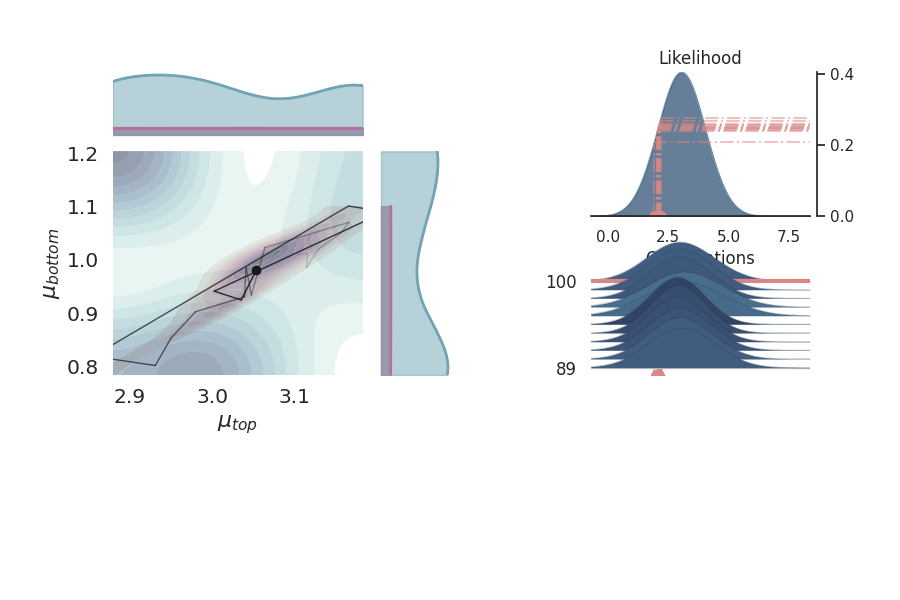
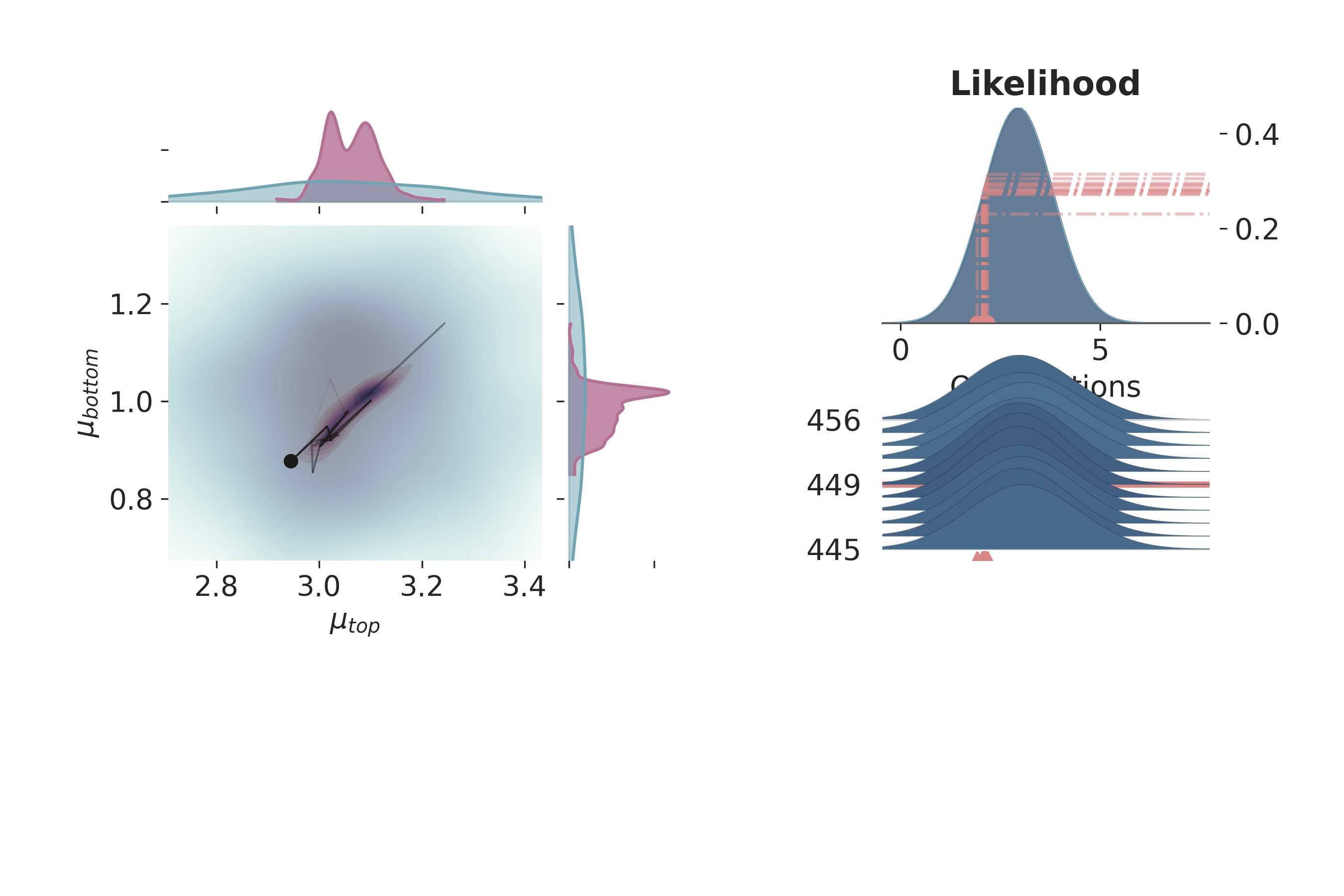
Posterior Distribution Visualization¶

This section provides a more detailed visualization of the posterior distributions of the parameters, integrating different aspects of the probabilistic model.

# Visualizing the posterior distributions
p = PlotPosterior(data)
p.create_figure(figsize=(9, 6), joyplot=True)
iteration = 450
p.plot_posterior(
    prior_var=['$\\mu_{top}$', '$\\mu_{bottom}$'],
    like_var=['$\\mu_{top}$', '$\\mu_{bottom}$'],
    obs='y_{thickness}',
    iteration=iteration,
    marginal_kwargs={
            "credible_interval" : .9999,
            'marginal_kwargs'   : {},
            'joint_kwargs'      : {
                    "bw"               : 1,
                    'contour'          : True,
                    'pcolormesh_kwargs': {}
            },
            "joint_kwargs_prior": {
                    'contour'          : False,
                    'pcolormesh_kwargs': {}
            }
    })
plt.show()

/home/leguark/gempy_probability/gempy_probability/plot_posterior.py:254: UserWarning: color is redundantly defined by the 'color' keyword argument and the fmt string "bo" (-> color='b'). The keyword argument will take precedence.
  self.axjoin.plot(theta1_val, theta2_val, 'bo', ms=6, color='k')

Pair Plot of Key Parameters¶

Pair plots are useful to visualize the relationships and correlations between different parameters. They help in understanding how parameters influence each other in the probabilistic model.

# Creating a pair plot for selected parameters
az.plot_pair(data, divergences=False, var_names=['$\\mu_{top}$', '$\\mu_{bottom}$'])
plt.show()

Total running time of the script: (0 minutes 36.612 seconds)

Gallery generated by Sphinx-Gallery