Note

Go to the end to download the full example code

2.2 - Including GemPy¶

Complex probabilistic model¶

import os
import numpy as np
import matplotlib.pyplot as plt
import torch
import pyro
import pyro.distributions as dist
from pyro.infer import MCMC, NUTS, Predictive
from pyro.infer.autoguide import init_to_mean
import gempy as gp
import gempy_engine
import gempy_viewer as gpv
from gempy.modules.data_manipulation.engine_factory import interpolation_input_from_structural_frame
from gempy_engine.core.backend_tensor import BackendTensor
import arviz as az

from gempy_engine.core.data.interpolation_input import InterpolationInput
from gempy_probability.plot_posterior import default_red, default_blue

# sphinx_gallery_thumbnail_number = -1

Set the data path

data_path = os.path.abspath('../')

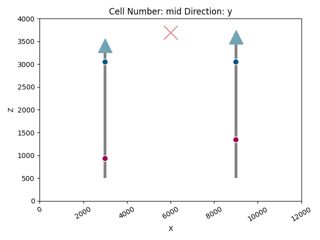
Define a function for plotting geological settings with wells

def plot_geo_setting_well(geo_model):
    """
    This function plots the geological settings along with the well locations.
    It uses gempy_viewer to create 2D plots of the model.
    """
    # Define well and device locations
    device_loc = np.array([[6e3, 0, 3700]])
    well_1 = 3.41e3
    well_2 = 3.6e3

    # Create a 2D plot
    p2d = gpv.plot_2d(geo_model, show_topography=False, legend=False, show=False)

    # Add well and device markers to the plot
    p2d.axes[0].scatter([3e3], [well_1], marker='^', s=400, c='#71a4b3', zorder=10)
    p2d.axes[0].scatter([9e3], [well_2], marker='^', s=400, c='#71a4b3', zorder=10)
    p2d.axes[0].scatter(device_loc[:, 0], device_loc[:, 2], marker='x', s=400, c='#DA8886', zorder=10)

    # Add vertical lines to represent wells
    p2d.axes[0].vlines(3e3, .5e3, well_1, linewidth=4, color='gray')
    p2d.axes[0].vlines(9e3, .5e3, well_2, linewidth=4, color='gray')

    # Show the plot
    p2d.fig.show()

Creating the Geological Model¶

Here we create a geological model using GemPy. The model defines the spatial extent, resolution, and geological information derived from orientations and surface points data.

geo_model = gp.create_geomodel(
    project_name='Wells',
    extent=[0, 12000, -500, 500, 0, 4000],
    refinement=3,
    importer_helper=gp.data.ImporterHelper(
        path_to_orientations=data_path + "/data/2-layers/2-layers_orientations.csv",
        path_to_surface_points=data_path + "/data/2-layers/2-layers_surface_points.csv"
    )
)

Configuring the Model¶

We configure the interpolation options for the geological model. These options determine how the model interpolates between data points.

geo_model.interpolation_options.uni_degree = 0
geo_model.interpolation_options.mesh_extraction = False
geo_model.interpolation_options.sigmoid_slope = 1100.

Setting up a Custom Grid¶

A custom grid is set for the model, defining specific points in space where geological formations will be evaluated.

x_loc = 6000
y_loc = 0
z_loc = np.linspace(0, 4000, 100)
xyz_coord = np.array([[x_loc, y_loc, z] for z in z_loc])
gp.set_custom_grid(geo_model.grid, xyz_coord=xyz_coord)

Active grids: GridTypes.NONE|CUSTOM|OCTREE

<gempy.core.data.grid_modules.grid_types.CustomGrid object at 0x7fb841b1b1c0>

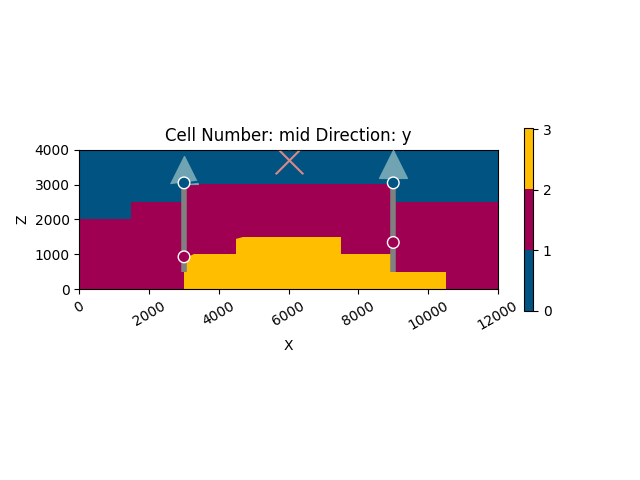
Plotting the Initial Geological Setting¶

Before running any probabilistic analysis, we first visualize the initial geological setting. This step ensures that our model is correctly set up with the initial data.

# Plot initial geological settings
plot_geo_setting_well(geo_model=geo_model)

Interpolating the Initial Guess¶

The model interpolates an initial guess for the geological formations. This step is crucial to provide a starting point for further probabilistic analysis.

gp.compute_model(
    gempy_model=geo_model,
    engine_config=gp.data.GemPyEngineConfig(backend=gp.data.AvailableBackends.numpy)
)
plot_geo_setting_well(geo_model=geo_model)

Setting Backend To: AvailableBackends.numpy

Probabilistic Geomodeling with Pyro¶

In this section, we introduce a probabilistic approach to geological modeling. By using Pyro, a probabilistic programming language, we define a model that integrates geological data with uncertainty quantification.

type_ = gempy_engine.core.data.interpolation_input.InterpolationInput
interpolation_input_copy: type_ = interpolation_input_from_structural_frame(geo_model)
sp_coords_copy = interpolation_input_copy.surface_points.sp_coords
# Change the backend to PyTorch for probabilistic modeling
BackendTensor.change_backend_gempy(engine_backend=gp.data.AvailableBackends.PYTORCH)

Setting Backend To: AvailableBackends.PYTORCH

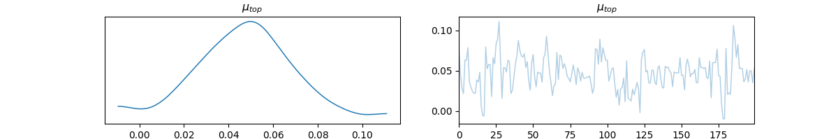
Defining the Probabilistic Model¶

The Pyro model represents the probabilistic aspects of the geological model. It defines a prior distribution for the top layer’s location and computes the thickness of the geological layer as an observed variable.

def model(y_obs_list):
    """
    This Pyro model represents the probabilistic aspects of the geological model.
    It defines a prior distribution for the top layer's location and
    computes the thickness of the geological layer as an observed variable.
    """
    # Define prior for the top layer's location:
    prior_mean = sp_coords_copy[0, 2]
    mu_top = pyro.sample(r'$\mu_{top}$', dist.Normal(prior_mean, torch.tensor(0.02, dtype=torch.float64)))

    # Update the model with the new top layer's location
    interpolation_input = interpolation_input_from_structural_frame(geo_model)
    interpolation_input.surface_points.sp_coords = torch.index_put(
        interpolation_input.surface_points.sp_coords,
        (torch.tensor([0]), torch.tensor([2])),
        mu_top
    )

    # Compute the geological model
    geo_model.solutions = gempy_engine.compute_model(
        interpolation_input=interpolation_input,
        options=geo_model.interpolation_options,
        data_descriptor=geo_model.input_data_descriptor,
        geophysics_input=geo_model.geophysics_input,
    )

    # Compute and observe the thickness of the geological layer
    simulated_well = geo_model.solutions.octrees_output[0].last_output_center.custom_grid_values
    thickness = simulated_well.sum()
    pyro.deterministic(r'$\mu_{thickness}$', thickness.detach())
    y_thickness = pyro.sample(r'$y_{thickness}$', dist.Normal(thickness, 50), obs=y_obs_list)

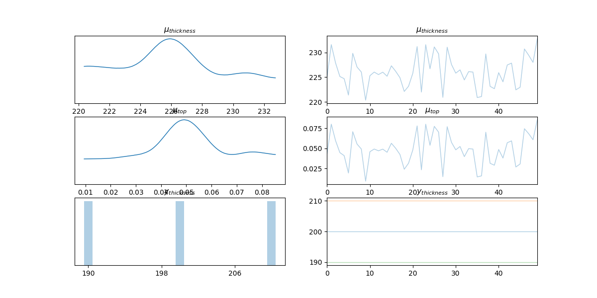
Running Prior Sampling and Visualization¶

Prior sampling is an essential step in probabilistic modeling. It helps in understanding the distribution of our prior assumptions before observing any data.

Prepare observation data

y_obs_list = torch.tensor([200, 210, 190])

Run prior sampling and visualization

prior = Predictive(model, num_samples=50)(y_obs_list)
data = az.from_pyro(prior=prior)
az.plot_trace(data.prior)
plt.show()

$\mu_{thickness}$, $\mu_{thickness}$, $\mu_{top}$, $\mu_{top}$, $y_{thickness}$, $y_{thickness}$

Sampling from the Posterior using MCMC¶

We use Markov Chain Monte Carlo (MCMC) with the NUTS (No-U-Turn Sampler) algorithm to sample from the posterior distribution. This gives us an understanding of the distribution of our model parameters after considering the observed data.

Run MCMC using NUTS to sample from the posterior

pyro.primitives.enable_validation(is_validate=True)
nuts_kernel = NUTS(model, step_size=0.0085, adapt_step_size=True, target_accept_prob=0.9, max_tree_depth=10, init_strategy=init_to_mean)
mcmc = MCMC(nuts_kernel, num_samples=200, warmup_steps=50, disable_validation=False)
mcmc.run(y_obs_list)

Warmup:   0%|          | 0/250 [00:00, ?it/s]
Warmup:   0%|          | 1/250 [00:00,  3.93it/s, step size=7.14e-02, acc. prob=0.041]
Warmup:   1%|          | 3/250 [00:00,  7.20it/s, step size=4.08e-03, acc. prob=0.347]
Warmup:   2%|▏         | 4/250 [00:00,  4.81it/s, step size=3.95e-03, acc. prob=0.510]
Warmup:   2%|▏         | 6/250 [00:01,  6.18it/s, step size=5.25e-03, acc. prob=0.673]
Warmup:   3%|▎         | 7/250 [00:01,  5.55it/s, step size=6.63e-03, acc. prob=0.719]
Warmup:   3%|▎         | 8/250 [00:01,  5.57it/s, step size=8.65e-03, acc. prob=0.754]
Warmup:   4%|▎         | 9/250 [00:01,  5.95it/s, step size=1.09e-02, acc. prob=0.779]
Warmup:   4%|▍         | 11/250 [00:01,  7.75it/s, step size=1.86e-02, acc. prob=0.816]
Warmup:   5%|▌         | 13/250 [00:01,  9.08it/s, step size=1.67e-02, acc. prob=0.826]
Warmup:   6%|▋         | 16/250 [00:01, 13.09it/s, step size=1.92e-02, acc. prob=0.842]
Warmup:   8%|▊         | 21/250 [00:02, 20.68it/s, step size=6.42e-03, acc. prob=0.836]
Warmup:  10%|▉         | 24/250 [00:02, 10.26it/s, step size=1.48e-02, acc. prob=0.855]
Warmup:  11%|█         | 27/250 [00:02, 12.67it/s, step size=2.76e-02, acc. prob=0.867]
Warmup:  12%|█▏        | 30/250 [00:02, 15.10it/s, step size=6.64e-03, acc. prob=0.852]
Warmup:  13%|█▎        | 33/250 [00:03, 14.05it/s, step size=1.45e-02, acc. prob=0.864]
Warmup:  14%|█▍        | 36/250 [00:03, 16.42it/s, step size=2.44e-02, acc. prob=0.872]
Warmup:  16%|█▌        | 39/250 [00:03, 15.66it/s, step size=1.02e-02, acc. prob=0.865]
Warmup:  16%|█▋        | 41/250 [00:03, 11.72it/s, step size=1.70e-02, acc. prob=0.871]
Warmup:  17%|█▋        | 43/250 [00:03, 12.39it/s, step size=2.55e-02, acc. prob=0.876]
Warmup:  18%|█▊        | 45/250 [00:04,  9.42it/s, step size=1.37e+01, acc. prob=0.876]
Warmup:  20%|██        | 50/250 [00:04, 14.07it/s, step size=1.09e+00, acc. prob=0.840]
Sample:  21%|██        | 52/250 [00:04, 14.38it/s, step size=1.09e+00, acc. prob=1.000]
Sample:  22%|██▏       | 55/250 [00:04, 15.72it/s, step size=1.09e+00, acc. prob=0.949]
Sample:  23%|██▎       | 58/250 [00:04, 18.09it/s, step size=1.09e+00, acc. prob=0.928]
Sample:  24%|██▍       | 61/250 [00:05, 18.34it/s, step size=1.09e+00, acc. prob=0.940]
Sample:  26%|██▌       | 64/250 [00:05, 18.55it/s, step size=1.09e+00, acc. prob=0.923]
Sample:  26%|██▋       | 66/250 [00:05, 17.06it/s, step size=1.09e+00, acc. prob=0.902]
Sample:  28%|██▊       | 69/250 [00:05, 19.32it/s, step size=1.09e+00, acc. prob=0.852]
Sample:  29%|██▉       | 72/250 [00:05, 17.40it/s, step size=1.09e+00, acc. prob=0.853]
Sample:  30%|██▉       | 74/250 [00:05, 17.07it/s, step size=1.09e+00, acc. prob=0.854]
Sample:  31%|███       | 77/250 [00:05, 17.48it/s, step size=1.09e+00, acc. prob=0.859]
Sample:  32%|███▏      | 79/250 [00:06, 16.25it/s, step size=1.09e+00, acc. prob=0.862]
Sample:  32%|███▏      | 81/250 [00:06, 15.94it/s, step size=1.09e+00, acc. prob=0.861]
Sample:  33%|███▎      | 83/250 [00:06, 15.34it/s, step size=1.09e+00, acc. prob=0.866]
Sample:  34%|███▍      | 86/250 [00:06, 16.47it/s, step size=1.09e+00, acc. prob=0.869]
Sample:  35%|███▌      | 88/250 [00:06, 17.23it/s, step size=1.09e+00, acc. prob=0.875]
Sample:  36%|███▋      | 91/250 [00:06, 20.27it/s, step size=1.09e+00, acc. prob=0.872]
Sample:  38%|███▊      | 94/250 [00:06, 20.37it/s, step size=1.09e+00, acc. prob=0.881]
Sample:  39%|███▉      | 97/250 [00:07, 21.87it/s, step size=1.09e+00, acc. prob=0.886]
Sample:  40%|████      | 100/250 [00:07, 20.86it/s, step size=1.09e+00, acc. prob=0.890]
Sample:  41%|████      | 103/250 [00:07, 20.04it/s, step size=1.09e+00, acc. prob=0.892]
Sample:  42%|████▏     | 106/250 [00:07, 19.18it/s, step size=1.09e+00, acc. prob=0.897]
Sample:  43%|████▎     | 108/250 [00:07, 18.46it/s, step size=1.09e+00, acc. prob=0.895]
Sample:  44%|████▍     | 111/250 [00:07, 20.74it/s, step size=1.09e+00, acc. prob=0.897]
Sample:  46%|████▌     | 114/250 [00:07, 20.13it/s, step size=1.09e+00, acc. prob=0.897]
Sample:  47%|████▋     | 117/250 [00:08, 19.78it/s, step size=1.09e+00, acc. prob=0.901]
Sample:  48%|████▊     | 120/250 [00:08, 18.16it/s, step size=1.09e+00, acc. prob=0.904]
Sample:  49%|████▉     | 123/250 [00:08, 20.40it/s, step size=1.09e+00, acc. prob=0.908]
Sample:  50%|█████     | 126/250 [00:08, 22.28it/s, step size=1.09e+00, acc. prob=0.910]
Sample:  52%|█████▏    | 129/250 [00:08, 19.66it/s, step size=1.09e+00, acc. prob=0.913]
Sample:  53%|█████▎    | 132/250 [00:08, 18.15it/s, step size=1.09e+00, acc. prob=0.914]
Sample:  54%|█████▎    | 134/250 [00:09, 16.64it/s, step size=1.09e+00, acc. prob=0.916]
Sample:  54%|█████▍    | 136/250 [00:09, 16.00it/s, step size=1.09e+00, acc. prob=0.913]
Sample:  55%|█████▌    | 138/250 [00:09, 16.05it/s, step size=1.09e+00, acc. prob=0.914]
Sample:  56%|█████▋    | 141/250 [00:09, 17.14it/s, step size=1.09e+00, acc. prob=0.916]
Sample:  58%|█████▊    | 144/250 [00:09, 17.42it/s, step size=1.09e+00, acc. prob=0.918]
Sample:  58%|█████▊    | 146/250 [00:09, 16.82it/s, step size=1.09e+00, acc. prob=0.915]
Sample:  59%|█████▉    | 148/250 [00:09, 16.03it/s, step size=1.09e+00, acc. prob=0.916]
Sample:  60%|██████    | 151/250 [00:09, 18.51it/s, step size=1.09e+00, acc. prob=0.915]
Sample:  61%|██████    | 153/250 [00:10, 17.09it/s, step size=1.09e+00, acc. prob=0.915]
Sample:  62%|██████▏   | 156/250 [00:10, 17.38it/s, step size=1.09e+00, acc. prob=0.916]
Sample:  64%|██████▍   | 160/250 [00:10, 21.19it/s, step size=1.09e+00, acc. prob=0.914]
Sample:  65%|██████▌   | 163/250 [00:10, 18.71it/s, step size=1.09e+00, acc. prob=0.914]
Sample:  66%|██████▌   | 165/250 [00:10, 17.57it/s, step size=1.09e+00, acc. prob=0.914]
Sample:  68%|██████▊   | 169/250 [00:10, 20.72it/s, step size=1.09e+00, acc. prob=0.914]
Sample:  69%|██████▉   | 173/250 [00:11, 22.70it/s, step size=1.09e+00, acc. prob=0.913]
Sample:  70%|███████   | 176/250 [00:11, 21.57it/s, step size=1.09e+00, acc. prob=0.914]
Sample:  72%|███████▏  | 179/250 [00:11, 21.13it/s, step size=1.09e+00, acc. prob=0.916]
Sample:  73%|███████▎  | 182/250 [00:11, 20.70it/s, step size=1.09e+00, acc. prob=0.912]
Sample:  74%|███████▍  | 185/250 [00:11, 17.95it/s, step size=1.09e+00, acc. prob=0.912]
Sample:  75%|███████▌  | 188/250 [00:11, 18.57it/s, step size=1.09e+00, acc. prob=0.913]
Sample:  76%|███████▋  | 191/250 [00:11, 20.83it/s, step size=1.09e+00, acc. prob=0.915]
Sample:  78%|███████▊  | 194/250 [00:12, 22.15it/s, step size=1.09e+00, acc. prob=0.916]
Sample:  79%|███████▉  | 197/250 [00:12, 21.34it/s, step size=1.09e+00, acc. prob=0.918]
Sample:  80%|████████  | 200/250 [00:12, 20.52it/s, step size=1.09e+00, acc. prob=0.917]
Sample:  81%|████████  | 203/250 [00:12, 19.84it/s, step size=1.09e+00, acc. prob=0.917]
Sample:  82%|████████▏ | 206/250 [00:12, 19.76it/s, step size=1.09e+00, acc. prob=0.919]
Sample:  84%|████████▎ | 209/250 [00:12, 17.75it/s, step size=1.09e+00, acc. prob=0.920]
Sample:  84%|████████▍ | 211/250 [00:13, 16.55it/s, step size=1.09e+00, acc. prob=0.920]
Sample:  86%|████████▌ | 214/250 [00:13, 17.24it/s, step size=1.09e+00, acc. prob=0.920]
Sample:  87%|████████▋ | 217/250 [00:13, 19.07it/s, step size=1.09e+00, acc. prob=0.920]
Sample:  88%|████████▊ | 219/250 [00:13, 18.08it/s, step size=1.09e+00, acc. prob=0.921]
Sample:  88%|████████▊ | 221/250 [00:13, 16.43it/s, step size=1.09e+00, acc. prob=0.920]
Sample:  90%|████████▉ | 224/250 [00:13, 18.86it/s, step size=1.09e+00, acc. prob=0.920]
Sample:  91%|█████████ | 227/250 [00:13, 18.39it/s, step size=1.09e+00, acc. prob=0.919]
Sample:  92%|█████████▏| 230/250 [00:14, 20.08it/s, step size=1.09e+00, acc. prob=0.915]
Sample:  93%|█████████▎| 233/250 [00:14, 18.05it/s, step size=1.09e+00, acc. prob=0.916]
Sample:  94%|█████████▍| 235/250 [00:14, 17.56it/s, step size=1.09e+00, acc. prob=0.915]
Sample:  95%|█████████▌| 238/250 [00:14, 20.01it/s, step size=1.09e+00, acc. prob=0.913]
Sample:  96%|█████████▋| 241/250 [00:14, 19.44it/s, step size=1.09e+00, acc. prob=0.912]
Sample:  98%|█████████▊| 244/250 [00:14, 18.84it/s, step size=1.09e+00, acc. prob=0.912]
Sample:  98%|█████████▊| 246/250 [00:14, 18.19it/s, step size=1.09e+00, acc. prob=0.913]
Sample:  99%|█████████▉| 248/250 [00:15, 17.27it/s, step size=1.09e+00, acc. prob=0.912]
Sample: 100%|██████████| 250/250 [00:15, 16.43it/s, step size=1.09e+00, acc. prob=0.912]
Sample: 100%|██████████| 250/250 [00:15, 16.44it/s, step size=1.09e+00, acc. prob=0.912]

Posterior Predictive Checks¶

After obtaining the posterior samples, we perform posterior predictive checks. This step is crucial to evaluate the performance and validity of our probabilistic model.

Sample from posterior predictive and visualize

posterior_samples = mcmc.get_samples()
posterior_predictive = Predictive(model, posterior_samples)(y_obs_list)
data = az.from_pyro(posterior=mcmc, prior=prior, posterior_predictive=posterior_predictive)
az.plot_trace(data)
plt.show()

$\mu_{top}$, $\mu_{top}$

/home/leguark/.virtualenvs/gempy_dependencies/lib/python3.10/site-packages/arviz/data/io_pyro.py:158: UserWarning: Could not get vectorized trace, log_likelihood group will be omitted. Check your model vectorization or set log_likelihood=False
  warnings.warn(

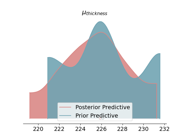
Density Plot of Posterior Predictive¶

A density plot provides a visual representation of the distribution of the posterior predictive checks. It helps in comparing the prior and posterior distributions and in assessing the impact of our observed data on the model.

Plot density of posterior predictive and prior predictive

az.plot_density(
    data=[data.posterior_predictive, data.prior_predictive],
    shade=.9,
    var_names=[r'$\mu_{thickness}$'],
    data_labels=["Posterior Predictive", "Prior Predictive"],
    colors=[default_red, default_blue],
)
plt.show()

$\mu_{thickness}$

Total running time of the script: (0 minutes 19.883 seconds)

Gallery generated by Sphinx-Gallery