Overview to Bayesian Inference

Model definition

Generally, models represent an abstraction of reality to answer a specific question, to fulfill a certain purpose, or to simulate (mimic) a proces or multiple processes. What models share is the aspiration to be as realistic as possible, so they can be used for prognoses and to better understand a real-world system.

Fitting of these models to acquired measurements or observations is called calibration and a standard procedure for improving a models reliability (to answer the question it was designed for).

Models can also be seen as a general descriptor of correlation of observations in multiple dimensions. Complex systems with generally sparse data coverage (e.g. the subsurface) are difficult to reliably encode from the real-world in the numerical abstraction, i.e. a computational model.

In a probabilistic framework, a model is a framework of different input distributions, which, as an output, has another probability distribution.

import io

import matplotlib.pyplot as plt
import pyro
import pyro.distributions as dist
import torch
from PIL import Image

# sphinx_gallery_thumbnail_number = -1

pyro.set_rng_seed(4003)

Simplest probabilistic modeling

Consider the simplest probabilistic model where the output \(y\) of a model is a distribution. Let’s assume, \(y\) is a normal distribution, described by a mean \(\mu\) and a standard deviation \(\sigma\). Usually, those are considered scalar values, but they themselves can be distributions. This will yield a change of the width and position of the normal distribution \(y\) with each iteration.

As a reminder, a normal distribution is defined as:

\[y = \frac{1}{\sigma \sqrt{2\pi}} \, e^{-\frac{(x - \mu)^2}{2 \sigma ^2}}\]

• \(\mu\): mean (Normal distribution)

• \(\sigma\): standard deviation (Gamma distribution, Gamma log-likelihood)

• \(y\): Normal distribution

With this constructed model, we are able to infer which model parameters will fit observations better by optimizing for regions with high density mass. In addition (or even substituting) to data observations, informative values like prior simulations or expert knowledge can pour into the construction of the first \(y\) distribution, the prior.

There isn’t a limitation about how “informative” a prior can or must be. Depending on the variance of the model’s parameters and on the number of observations, a model will be more prior driven or data driven.

Let’s set up a Pyro model using the thickness_observation from above as observations and with \(\mu\) and \(\sigma\) being:

• \(\mu = \text{Normal distribution with mean } 2.08 \text{ and standard deviation } 0.07\)

• \(\sigma = \text{Gamma distribution with } \alpha = 0.3 \text{ and } \beta = 3\)

• \(y = \text{Normal distribution with } \mu, \sigma \text{ and thickness_observation_list as observations}\)

A Gamma distribution can also be expressed by mean and standard deviation with \(\alpha = \frac{\mu^2}{\sigma^2}\) and \(\beta = \frac{\mu}{\sigma^2}\).

def model(distributions_family, data):
    if distributions_family == "normal_distribution":
        param_mean = pyro.param('$\\mu_{prior}$', torch.tensor(2.07))
        param_std = pyro.param('$\\sigma_{prior}$', torch.tensor(0.07), constraint=dist.constraints.positive)
        mu = pyro.sample('$\\mu_{likelihood}$', dist.Normal(param_mean, param_std))
    elif distributions_family in "uniform_distribution":
        param_low = pyro.param('$\\mu_{prior}$', torch.tensor(0))
        param_high = pyro.param('$\\sigma_{prior}$', torch.tensor(10))
        mu = pyro.sample('$\\mu_{likelihood}$', dist.Uniform(param_low, param_high))
    else:
        raise ValueError("distributions_family must be either 'normal_distribution' or 'uniform_distribution'")
    param_concentration = pyro.param('$\\alpha_{prior}$', torch.tensor(0.3), constraint=dist.constraints.positive)
    param_rate = pyro.param('$\\beta_{prior}$', torch.tensor(3), constraint=dist.constraints.positive)

    sigma = pyro.sample('$\\sigma_{likelihood}$', dist.Gamma(param_concentration, param_rate))
    y = pyro.sample('$y$', dist.Normal(mu, sigma), obs=data)
    return y

y_obs = torch.tensor([2.12])
y_obs_list = torch.tensor([2.12, 2.06, 2.08, 2.05, 2.08, 2.09,
                           2.19, 2.07, 2.16, 2.11, 2.13, 1.92])

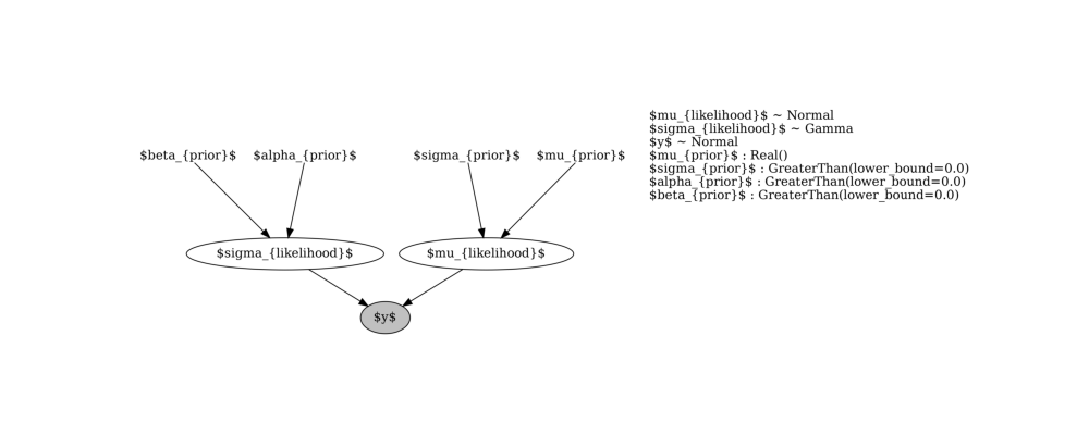
Render the model as a graph

graph = pyro.render_model(
    model=model,
    model_args=("normal_distribution", y_obs_list,),
    render_params= True,
    render_distributions=True
)
graph.attr(dpi='300')
# Convert the graph to a PNG image format
s = graph.pipe(format='png')

# Open the image with PIL
image = Image.open(io.BytesIO(s))

# Plot the image with matplotlib
plt.figure(figsize=(10, 4))
plt.imshow(image)
plt.axis('off')  # Turn off axis
plt.show()

Next:

• Several Observations: (Normal Prior, several observations)

• One Observation: (Normal Prior, single observation)

License

The code in this case study is copyrighted by Miguel de la Varga and licensed under the new BSD (3-clause) license:

https://opensource.org/licenses/BSD-3-Clause

The text and figures in this case study are copyrighted by Miguel de la Varga and licensed under the CC BY-NC 4.0 license:

https://creativecommons.org/licenses/by-nc/4.0/ Make sure to replace the links with actual hyperlinks if you’re using a platform that supports it (e.g., Markdown or HTML). Otherwise, the plain URLs work fine for plain text.